Data Structures/Graphs
From
Data Structures
Introduction - Asymptotic Notation - Arrays - List Structures & Iterators
Stacks & Queues - Trees - Min & Max Heaps - Graphs
Hash Tables - Sets - Tradeoffs
Contents |
Graphs
A graph is a collection of vertices (also called nodes) and edges (also called arcs) that connect these vertices. A graph is a generalization of the tree structure, where instead of a strict parent/child relationship between tree nodes, any kind of complex relationships between the nodes can be represented.
Directed Graphs
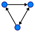
The number of edges with one endpoint on a given vertex is called that vertex's degree. In a directed graph, the number of edges that point to a given vertex is called its in-degree, and the number that point from it is called its out-degree. Often, we may want to be able to distinguish between different nodes and edges. We can associate labels with either. We call such a graph labeled.
Directed Graph Operations
make-graph(): graph- Create a new graph, initially with no nodes or edges.
make-vertex(graph G, element value): vertex- Create a new vertex, with the given value.
make-edge(vertex u, vertex v): edge- Create an edge between u and v. In a directed graph, the edge will flow from u to v.
get-edges(vertex v): edge-set- Returns the set of edges flowing from v
get-neighbors(vertex v): vertex-set- Returns the set of vertexes connected to v
[TODO: also need undirected graph abstraction in that section, and also find a better set of operations-- the key to finding good operations is seeing what the algorithms that use graphs actually need]
We can use graphs to represent relationships between objects. For example, the popular game "Six Degrees of Kevin Bacon" can be modeled by a graph, in particular, a labeled undirected graph. Each actor becomes a node, labeled by the actor's name. Nodes are connected by an edge when the two actors appeared together in some movie. We can label this edge by the name of the movie. Then the problem of finding a path from any actor to Kevin Bacon in six or less steps easily reduces to the Single Source Shortest Path problem found in the companion Algorithms book. The Oracle of Bacon at the University of Virginia has actually implemented this algorithm and can tell you the path from any actor to Kevin Bacon in a few clicks[1].
Undirected Graphs
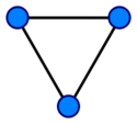
In a directed graph, the edges point from one vertex to another, while in an undirected graph, they merely connect two vertices.
Weighted Graphs
We may also want to associate some cost or weight to the traversal of an edge. When we add this information, the graph is called weighted. An example of a weighted graph would be the distance between the capitals of a set of countries.
Directed and undirected graphs may both be weighted. The operations on a weighted graph are the same with addition of a weight parameter during edge creation:
Weighted Graph Operations (an extension of undirected/directed graph operations)
make-edge(vertex u, vertex v, weight w): edge- Create an edge between u and v with weight w. In a directed graph, the edge will flow from u to v.
Graph Representations
Adjacency Matrix Representation
An adjacency matrix is one of the two common ways to represent a graph. The adjacency matrix shows which nodes are adjacent to one another. Two nodes are adjacent if there is an edge connecting them. In the case of a directed graph, if node j is adjacent to node i, there is an edge from i to j. In other words, if j is adjacent to i, you can get from i to j by traversing one edge. For a given graph with n nodes, the adjacency matrix will have dimensions of  . For an unweighted graph, the adjacency matrix will be populated with boolean values.
For any given node i, you can determine its adjacent nodes by looking at row  of the adjacency matrix. A value of true at
  indicates that there is an edge from node i to node j, and false indicating no edge. In an undirected graph, the values of
  and
and  will be equal. In a weighted graph, the boolean values will be replaced by the weight of the edge connecting the two nodes, with a special value that indicates the absence of an edge.
The memory use of an adjacency matrix is O(n2).
Adjacency List Representation
The adjacency list is another common representation of a graph. There are many ways to implement this adjacency representation. One way is to have the graph maintain a list of lists, in which the first list is a list of indices corresponding to each node in the graph. Each of these refer to another list that stores a the index of each adjacent node to this one. It might also be useful to associate the weight of each link with the adjacent node in this list.
Example: An undirected graph contains four nodes 1, 2, 3 and 4. 1 is linked to 2 and 3. 2 is linked to 3. 3 is linked to 4.
1 - [2, 3]
2 - [1, 3]
3 - [1, 2, 4]
4 - [3]
It might be useful to store the list of all the nodes in the graph in a hash table. The keys then would correspond to the indices of each node and the value would be a reference to the list of adjacent node indecies.
Another implementation might require that each node keep a list of its adjacent nodes.
Graph Traversals
Depth-First Search
Start at vertex v, visit its neighbour w, then w's neighbour y and keep going until reach 'a dead end' then iterate back and visit nodes reachable from second last visited vertex and keep applying the same principle.
[TODO: depth-first search -- with compelling example]
// Search in the subgraph for a node matching 'criteria'. Do not re-examine
// nodes listed in 'visited' which have already been tested.
GraphNode depth_first_search(GraphNode node, Predicate criteria, VisitedSet visited) {
 // Check that we haven't already visited this part of the graph
 if (visited.contains(node)) {
   return null;
 }
 visited.insert(node);
 // Test to see if this node satifies the criteria
 if (criteria.apply(node.value)) {
   return node;
 }
 // Search adjacent nodes for a match
 for (adjacent in node.adjacentnodes()) {
   GraphNode ret = depth_first_search(adjacent, criteria, visited);
   if (ret != null) {
     return ret;
   }
 }
 // Give up - not in this part of the graph
 return null;
}
Breadth-First Search
Breadth first search visits the nodes neighbours and then the univisited neighbours of the neighbours etc. If it starts on vertex a it will go to all vertices that have an edge from a. If some points are not reachable it will have to start another BFS from a new vertex.
[TODO: breadth-first search -- with compelling example]
[TODO: topological sort -- with compelling example]


