Data Structures/All Chapters
From
Data Structures
Introduction - Asymptotic Notation - Arrays - List Structures & Iterators
Stacks & Queues - Trees - Min & Max Heaps - Graphs
Hash Tables - Sets - Tradeoffs
Computers can store and process vast amounts of data. Formal data structures enable a programmer to mentally structure large amounts of data into conceptually manageable relationships.
Sometimes we use data structures to allow us to do more: for example, to accomplish fast searching or sorting of data. Other times, we use data structures so that we can do less: for example, the concept of the stack is a limited form of a more general data structure. These limitations provide us with guarantees that allow us to reason about our programs more easily. Data structures also provide guarantees about algorithmic complexity — choosing an appropriate data structure for a job is crucial for writing good software.
Because data structures are higher-level abstractions, they present to us operations on groups of data, such as adding an item to a list, or looking up the highest-priority item in a queue. When a data structure provides operations, we can call the data structure an abstract data type (sometimes abbreviated as ADT). Abstract data types can minimize dependencies in your code, which is important when your code needs to be changed. Because you are abstracted away from lower-level details, some of the higher-level commonalities one data structure shares with a different data structure can be used to replace one with the other.
Our programming languages come equipped with a set of built-in types, such as integers and floating-point numbers, that allow us to work with data objects for which the machine's processor has native support. These built-in types are abstractions of what the processor actually provides because built-in types hide details both about their execution and limitations.
For example, when we use a floating-point number we are primarily concerned with its value and the operations that can be applied to it. Consider computing the length of a hypotenuse:
let c := sqrt(a * a + b * b)
The machine code generated from the above would use common patterns for computing these values and accumulating the result. In fact, these patterns are so repetitious that high-level languages were created to avoid this redundancy and to allow programmers to think about what value was computed instead of how it was computed.
Two useful and related concepts are at play here:
- Abstraction is when common patterns are grouped together under a single name and then parameterized, in order to achieve a higher-level understanding of that pattern. For example, the multiplication operation requires two source values and writes the product of those two values to a given destination. The operation is parameterized by both the two sources and the single destination.
- Encapsulation is a mechanism to hide the implementation details of an abstraction away from the users of the abstraction. When we multiply numbers, for example, we don't need to know the technique actually used by the processor, we just need to know its properties.
A programming language is both an abstraction of a machine and a tool to encapsulate-away the machine's inner details. For example, a program written in a programming language can be compiled to several different machine architectures when that programming language sufficiently encapsulates the user away from any one machine.
In this book, we take the abstraction and encapsulation that our programming languages provide a step further: When applications get to be more complex, the abstractions programming languages provide become too low-level to effectively manage. Thus, we build our own abstractions on top of these lower-level constructs. We can even build further abstractions on top of those abstractions. Each time we build upwards, we lose access to the lower-level implementation details. While losing such access might sound like a bad trade off, it is actually quite a bargain: We are primarily concerned with solving the problem at hand rather than with any trivial decisions that could have just as arbitrarily been replaced with a different decision. When we can think on higher levels, we relieve ourselves of these burdens.
Each data structure that we cover in this book can be thought of as a single unit that has a set of values and a set of operations that can be performed to either access or change these values. The data structure itself can be understood as a set of the data structure's operations together with each operation's properties (i.e., what the operation does and how long we could expect it to take).
The Node
The first data structure we look at is the node structure. A node is simply a container for a value, plus a pointer to a "next" node (which may be null).
Node<Element> Operations
make-node(Element v, Node next): Node
- Create a new node, with v as its contained value and next as the value of the next pointer
get-value(Node n): Element
- Returns the value contained in node n
get-next(Node n): Node
- Returns the value of node n's next pointer
set-value(Node n, Element v)
- Sets the contained value of n to be v
set-next(Node n, Node new-next)
- Sets the value of node n's next pointer to be new-next
All operations can be performed in time that is O(1).
Examples of the "Element" type can be: numbers, strings, objects, functions, or even other nodes. Essentially, any type that has values at all in the language.
The above is an abstraction of a structure:
  structure node {
    element value     // holds the value
    node next         // pointer to the next node; possibly null
  }
In some languages, structures are called records or classes. Some other languages provide no direct support for structures, but instead allow them to be built from other constructs (such as tuples or lists).
Here, we are only concerned that nodes contain values of some form, so we simply say its type is "element" because the type is not important. In some programming languages no type ever needs to be specified (as in dynamically typed languages, like Scheme, Smalltalk or Python). In other languages the type might need to be restricted to integer or string (as in statically typed languages like C). In still other languages, the decision of the type of the contained element can be delayed until the type is actually used (as in languages that support generic types, like C++ and Java). In any of these cases, translating the pseudocode into your own language should be relatively simple.
Each of the node operations specified can be implemented quite easily:
// Create a new node, with v as its contained value and next as
// the value of the next pointer
function make-node(v, node next): node
  let result := new node {v, next}
  return result
end

// Returns the value contained in node n
function get-value(node n): element
  return n.value
end

// Returns the value of node n's next pointer
function get-next(node n): node
  return n.next
end

// Sets the contained value of n to be v
function set-value(node n, v)
  n.value := v
end

// Sets the value of node n's next pointer to be new-next
function set-next(node n, new-next)
  n.next := new-next
end
Principally, we are more concerned with the operations and the implementation strategy than we are with the structure itself and the low-level implementation. For example, we are more concerned about the time requirement specified, which states that all operations take time that is O(1). The above implementation meets this criteria, because the length of time each operation takes is constant. Another way to think of constant time operations is to think of them as operations whose analysis is not dependent on any variable. (The notation O(1) is mathematically defined in the next chapter. For now, it is safe to assume it just means constant time.)
Because a node is just a container both for a value and container to a pointer to another node, it shouldn't be surprising how trivial the node data structure itself (and its implementation) is.
Building a Chain from Nodes
Although the node structure is simple, it actually allows us to compute things that we couldn't have computed with just fixed-size integers alone.
But first, we'll look at a program that doesn't need to use nodes. The following program will read in (from an input stream; which can either be from the user or a file) a series of numbers until the end-of-file is reached and then output what the largest number is and the average of all numbers:
program(input-stream in, output-stream out) let total := 0 let count := 0 let largest :=while has-next-integer(in): let i := read-integer(in) total := total + i count := count + 1 largest := max(largest, i) repeat println out "Maximum: " largest if count != 0: println out "Average: " (total / count) fi end
But now consider solving a similar task: read in a series of numbers until the end-of-file is reached, and output the largest number and the average of all numbers that evenly divide the largest number. This problem is different because it's possible the largest number will be the last one entered: if we are to compute the average of all numbers that divide that number, we'll need to somehow remember all of them. We could use variables to remember the previous numbers, but variables would only help us solve the problem when there aren't too many numbers entered.
For example, suppose we were to give ourselves 200 variables to hold the state input by the user. And further suppose that each of the 200 variables had 64-bits. Even if we were very clever with our program, it could only compute results for  different types of input. While this is a very large number of combinations, a list of 300 64-bit numbers would require even more combinations to be properly encoded. (In general, the problem is said to require linear space. All programs that need only a finite number of variables can be solved in constant space.)
Instead of building-in limitations that complicate coding (such as having only a constant number of variables), we can use the properties of the node abstraction to allow us to remember as many numbers as our computer can hold:
program(input-stream in, output-stream out) let largest :=
Above, if n integers are successfully read there will be n calls made to make-node. This will require n nodes to be made (which require enough space to hold the value and next fields of each node, plus internal memory management overhead), so the memory requirements will be on the order of O(n). Similarly, we construct this chain of nodes and then iterate over the chain again, which will require O(n) steps to make the chain, and then another O(n) steps to iterate over it.
Note that when we iterate the numbers in the chain, we are actually looking at them in reverse order. For example, assume the numbers input to our program are 4, 7, 6, 30, and 15. After EOF is reached, the nodes chain will look like this:
Such chains are more commonly referred to as linked-lists. However, we generally prefer to think in terms of lists or sequences, which aren't as low-level: the linking concept is just an implementation detail. While a list can be made with a chain, in this book we cover several other ways to make a list. For the moment, we care more about the abstraction capabilities of the node than we do about one of the ways it is used.
The above algorithm only uses the make-node, get-value, and get-next functions. If we use set-next we can change the algorithm to generate the chain so that it keeps the original ordering (instead of reversing it). [TODO: pseudocode to do so; also TODO; should probably think of compelling, but not too-advanced, use of set-value.]
program (input-stream in, output-stream out) let largest :=
The Principle of Induction
The chains we can build from nodes are a demonstration of the principle of mathematical induction:
Mathematical Induction
|
For example, let the property P(n) be the statement that "you can make a chain that holds n numbers". This is a property of natural numbers, because the sentence makes sense for specific values of n:
- you can make a chain that holds 5 numbers
- you can make a chain that holds 100 numbers
- you can make a chain that holds 1,000,000 numbers
Instead of proving that we can make chains of length 5, 100, and one million, we'd rather prove the general statement P(n) instead. Step 2 above is called the Inductive Hypothesis; let's show that we can prove it:
- Assume that P(n) holds. That is, that we can make a chain of n elements. Now we must show that P(n + 1) holds.
- Assume
chainis the first node of the n-element chain. Assumeiis some number that we'd like to add to the chain to make an n + 1 length chain. - The following code can accomplish this for us:
let bigger-chain := make-node(i, chain)
- Here, we have the new number
ithat is now the contained value of the first link of thebigger-chain. Ifchainhad n elements, thenbigger-chainmust have n + 1 elements.
Step 3 above is called the Base Case, let's show that we can prove it:
- We must show that P(1) holds. That is, that we can make a chain of one element.
- The following code can accomplish this for us:
let chain := make-node(i, null)
The principle of induction says, then, that we have proven that we can make a chain of n elements for all value of  . How is this so? Probably the best way to think of induction is that it's actually a way of creating a formula to describe an infinite number of proofs. After we prove that the statement is true for P(1), the base case, we can apply the inductive hypothesis to that fact to show that P(2) holds. Since we now know that P(2) holds, we can apply the inductive hypothesis again to show that P(3) must hold. The principle says that there is nothing to stop us from doing this repeatedly, so we should assume it holds for all cases.
Induction may sound like a strange way to prove things, but it's a very useful technique. What makes the technique so useful is that it can take a hard sounding statement like "prove P(n) holds for all " and break it into two smaller, easier to prove statements. Typically base cases are easy to prove because they are not general statements at all. Most of the proof work is usually in the inductive hypothesis, which can often require clever ways of reformulating the statement to "attach on" a proof of the n + 1 case.
You can think of the contained value of a node as a base case, while the next pointer of the node as the inductive hypothesis. Just as in mathematical induction, we can break the hard problem of storing an arbitrary number of elements into an easier problem of just storing one element and then having a mechanism to attach on further elements.
Induction on a Summation
The next example of induction we consider is more algebraic in nature:
Let's say we are given the formula  and we want to prove that this formula gives us the sum of the first n numbers. As a first attempt, we might try to just show that this is true for 1
 ,
,
for 2
 ,
,
for 3
and so on, however we'd quickly realize that our so called proof would take infinitely long to write out! Even if you carried out this proof and showed it to be true for the first billion numbers, that doesn't nescessarily mean that it would be true for one billion and one or even a hundred billion. This is a strong hint that maybe induction would be useful here.
Let's say we want to prove that the given formula really does give the sum of the first n numbers using induction. The first step is to prove the base case; i.e. we have to show that it is true when n = 1. This is relatively easy; we just substitute 1 for the variable n and we get ( ), which shows that the formula is correct when n = 1.
Now for the inductive step. We have to show that if the formula is true for j, it is also true for j + 1. To phrase it another way, assuming we've already proven that the sum from 1 to (j) is  , we want to prove that the sum from 1 to (j+1) is
  . Note that those two formulas came about just by replacing n with (j) and (j+1) respectively.
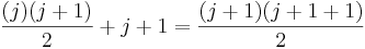
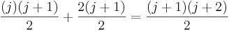
To prove this inductive step, first note that to calculate the sum from 1 to j+1, you can just calculate the sum from 1 to j, then add j+1 to it. We already have a formula for the sum from 1 to j, and when we add j+1 to that formula, we get this new formula:  . So to actually complete the proof, all we'd need to do is show that
  .
.
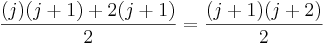
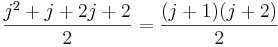
We can show the above equation is true via a few simplification steps:
Data Structures
Introduction - Asymptotic Notation - Arrays - List Structures & Iterators
Stacks & Queues - Trees - Min & Max Heaps - Graphs
Hash Tables - Sets - Tradeoffs
Data Structures
Introduction - Asymptotic Notation - Arrays - List Structures & Iterators
Stacks & Queues - Trees - Min & Max Heaps - Graphs
Hash Tables - Sets - Tradeoffs
Asymptotic Notation
Introduction
A problem may have numerous algorithmic solutions. In order to choose the best algorithm for a particular task, you need to be able to judge how long a particular solution will take to run. Or, more accurately, you need to be able to judge how long two solutions will take to run, and choose the better of the two. You don't need to know how many minutes and seconds they will take, but you do need some way to compare algorithms against one another.
Asymptotic complexity is a way of expressing the main component of the cost of an algorithm, using idealized units of computational work. Consider, for example, the algorithm for sorting a deck of cards, which proceeds by repeatedly searching through the deck for the lowest card. The asymptotic complexity of this algorithm is the square of the number of cards in the deck. This quadratic behavior is the main term in the complexity formula, it says, e.g., if you double the size of the deck, then the work is roughly quadrupled.
The exact formula for the cost is more complex, and contains more details than are needed to understand the essential complexity of the algorithm. With our deck of cards, in the worst case, the deck would start out reverse-sorted, so our scans would have to go all the way to the end. The first scan would involve scanning 52 cards, the next would take 51, etc. So the cost formula is 52 + 51 + ... + 1. generally, letting N be the number of cards, the formula is 1 + 2 + ... + N, which equals (N + 1) * (N / 2) = (N2 + N) / 2 = (1 / 2)N2 + N / 2. But the N^2 term dominates the expression, and this is what is key for comparing algorithm costs. (This is in fact an expensive algorithm; the best sorting algorithms run in sub-quadratic time.)
Asymptotically speaking, in the limit as N tends towards infinity, 1 + 2 + ... + N gets closer and closer to the pure quadratic function (1/2) N^2. And what difference does the constant factor of 1/2 make, at this level of abstraction. So the behavior is said to be O(n2).
Now let us consider how we would go about comparing the complexity of two algorithms. Let f(n) be the cost, in the worst case, of one algorithm, expressed as a function of the input size n, and g(n) be the cost function for the other algorithm. E.g., for sorting algorithms, f(10) and g(10) would be the maximum number of steps that the algorithms would take on a list of 10 items. If, for all values of n >= 0, f(n) is less than or equal to g(n), then the algorithm with complexity function f is strictly faster. But, generally speaking, our concern for computational cost is for the cases with large inputs; so the comparison of f(n) and g(n) for small values of n is less significant than the "long term" comparison of f(n) and g(n), for n larger than some threshold.
Note that we have been speaking about bounds on the performance of algorithms, rather than giving exact speeds. The actual number of steps required to sort our deck of cards (with our naive quadratic algorithm) will depend upon the order in which the cards begin. The actual time to perform each of our steps will depend upon our processor speed, the condition of our processor cache, etc., etc. It's all very complicated in the concrete details, and moreover not relevant to the essence of the algorithm.
Big-O Notation
Definition
Big-O is the formal method of expressing the upper bound of an algorithm's running time. It's a measure of the longest amount of time it could possibly take for the algorithm to complete.
More formally, for non-negative functions, f(n) and g(n), if there exists an integer n0 and a constant c > 0 such that for all integers n > n0, f(n) ≤ cg(n), then f(n) is Big O of g(n). This is denoted as "f(n) = O(g(n))". If graphed, g(n) serves as an upper bound to the curve you are analyzing, f(n).
Theory Examples
So, let's take an example of Big-O. Say that f(n) = 2n + 8, and g(n) = n2. Can we find a constant c, so that 2n + 8 <= n2? The number 4 works here, giving us 16 <= 16. For any number c greater than 4, this will still work. Since we're trying to generalize this for large values of n, and small values (1, 2, 3) aren't that important, we can say that f(n) is generally faster than g(n); that is, f(n) is bound by g(n), and will always be less than it.
It could then be said that f(n) runs in O(n2) time: "f-of-n runs in Big-O of n-squared time".
To find the upper bound - the Big-O time - assuming we know that f(n) is equal to (exactly) 2n + 8, we can take a few shortcuts. For example, we can remove all constants from the runtime; eventually, at some value of c, they become irrelevant. This makes f(n) = 2n. Also, for convenience of comparison, we remove constant multipliers; in this case, the 2. This makes f(n) = n. It could also be said that f(n) runs in O(n) time; that lets us put a tighter (closer) upper bound onto the estimate.
Practical Examples
O(n): printing a list of n items to the screen, looking at each item once. O(ln n): also "log n", taking a list of items, cutting it in half repeatedly until there's only one item left. O(n2): taking a list of n items, and comparing every item to every other item.
Big-Omega Notation
For non-negative functions, f(n) and g(n), if there exists an integer n0 and a constant c > 0 such that for all integers n > n0, f(n) ≥ cg(n), then f(n) is omega of g(n). This is denoted as "f(n) = Ω(g(n))".
This is almost the same definition as Big Oh, except that "f(n) ≥ cg(n)", this makes g(n) a lower bound function, instead of an upper bound function. It describes the best that can happen for a given data size.
Theta Notation
- Theta Notation
- For non-negative functions, f(n) and g(n), f(n) is theta of g(n) if and only if f(n) = O(g(n)) and f(n) = Ω(g(n)). This is denoted as "f(n) = Θ(g(n))".
This is basically saying that the function, f(n) is bounded both from the top and bottom by the same function, g(n).
Little-O Notation
For non-negative functions, f(n) and g(n), f(n) is little o of g(n) if and only if f(n) = O(g(n)), but f(n) ≠ Θ(g(n)). This is denoted as "f(n) = o(g(n))".
This represents a loose bounding version of Big O. g(n) bounds from the top, but it does not bound the bottom.
Little Omega Notation
For non-negative functions, f(n) and g(n), f(n) is little omega of g(n) if and only if f(n) = Ω(g(n)), but f(n) ≠ Θ(g(n)). This is denoted as "f(n) = ω(g(n))".
Much like Little Oh, this is the equivalent for Big Omega. g(n) is a loose lower boundary of the function f(n); it bounds from the bottom, but not from the top.
How asymptotic notation relates to analyzing complexity
Temporal comparison is not the only issue in algorithms. There are space issues as well. Generally, a trade off between time and space is noticed in algorithms. Asymptotic notation empowers you to make that trade off. If you think of the amount of time and space your algorithm uses as a function of your data over time or space (time and space are usually analyzed separately), you can analyze how the time and space is handled when you introduce more data to your program.
This is important in data structures because you want a structure that behaves efficiently as you increase the amount of data it handles. Keep in mind though that algorithms that are efficient with large amounts of data are not always simple and efficient for small amounts of data. So if you know you are working with only a small amount of data and you have concerns for speed and code space, a trade off can be made for a function that does not behave well for large amounts of data.
A few examples of asymptotic notation
Generally, we use asymptotic notation as a convenient way to examine what can happen in a function in the worst case or in the best case. For example, if you want to write a function that searches through an array of numbers and returns the smallest one:
function find-min(array a[1..n]) let j :=for i := 1 to n: j := min(j, a[i]) repeat return j end
Regardless of how big or small the array is, every time we run find-min, we have to initialize the i and j integer variables and return j at the end. Therefore, we can just think of those parts of the function as constant and ignore them.
So, how can we use asymptotic notation to discuss the find-min function? If we search through an array with 87 elements, then the for loop iterates 87 times, even if the very first element we hit turns out to be the minimum. Likewise, for n elements, the for loop iterates n times. Therefore we say the function runs in time O(n).
What about this function:
function find-min-plus-max(array a[1..n]) // First, find the smallest element in the array let j :=
What's the running time for find-min-plus-max? There are two for loops, that each iterate n times, so the running time is clearly O(2n). Because 2 is a constant, we throw it away and write the running time as O(n). Why can you do this? If you recall the definition of Big-O notation, the function whose bound you're testing can be multiplied by some constant. If f(x) = 2x, we can see that if g(x) = x, then the Big-O condition holds. Thus O(2n) = O(n). This rule is general for the various asymptotic notations.
Data Structures
Introduction - Asymptotic Notation - Arrays - List Structures & Iterators
Stacks & Queues - Trees - Min & Max Heaps - Graphs
Hash Tables - Sets - Tradeoffs
Data Structures
Introduction - Asymptotic Notation - Arrays - List Structures & Iterators
Stacks & Queues - Trees - Min & Max Heaps - Graphs
Hash Tables - Sets - Tradeoffs
Arrays
An array is a particular method of storing elements of indexed data. Elements of data are stored sequentially in blocks within the array. Each element is referenced by an index, or subscript.
The index is usually a number used to address an element in the array. For example, if you were storing information about each day in August, you would create an array with an index capable of addressing 31 values -- one for each day of the month. Indexing rules are language dependent, however most languages use either 0 or 1 as the first element of an array.
The concept of an array can be daunting to the uninitiated, but it is really quite simple. Think of a notebook with pages numbered 1 through 12. Each page may or may not contain information on it. The notebook is an array of pages. Each page is an element of the array 'notebook'. Programmatically, you would retrieve information from a page by referring to its number or subscript, i.e., notebook(4) would refer to the contents of page 4 of the array notebook.
The notebook (array) contains 12 pages (elements)
Arrays can also be multidimensional - instead of accessing an element of a one-dimensional list, elements are accessed by two or more indices, as from a matrix or tensor.
Multidimensional arrays are as simple as our notebook example above. To envision a multidimensional array, think of a calendar. Each page of the calendar, 1 through 12, is an element, representing a month, which contains approximately 30 elements, which represent days. Each day may or may not have information in it. Programmatically then, calendar(4,15) would refer to the 4th month, 15th day. Thus we have a two-dimensional array. To envision a three-dimensional array, break each day up into 24 hours. Now calendar(4,15,9) would refer to 4th month, 15th day, 9th hour.

A simple 6 element by 4 element array
Array<Element> Operations
make-array(integer n): Array
- Create an array of elements indexed from 0 to n − 1, inclusive. The number of elements in the array, also known as the size of the array, is n.
get-value-at(Array a, integer index): Element
- Returns the value of the element at the given index. The value of index must be in bounds: 0 <= index <= (n - 1). This operation is also known as subscripting.
set-value-at(Array a, integer index, Element new-value)
- Sets the element of the array at the given index to be equal to new-value.
Arrays guarantee constant time read and write access, O(1), however many lookup operations (find_min, find_max, find_index) of an instance of an element are linear time, O(n). Arrays are very efficient in most languages, as operations compute the address of an element via a simple formula based on the base address element of the array.
The implementation of arrays differ greatly between languages: some languages allow arrays to be resized automatically, or to even contain elements of differing types (such as Perl). Other languages are very strict and require the type and length information of an array to be known at run time (such as C).
Arrays typically map directly to contiguous storage locations within your computers memory and are therefore the "natural" storage structure for most higher level languages.
Simple linear arrays are the basis for most of the other data structures. Many languages do not allow you to allocate any structure except an array, everything else must be implemented on top of the array. The exception is the linked list, that is typically implemented as individually allocated objects, but it is possible to implement a linked list within an array.
Type
The array index needs to be of some type. Usually, the standard integer type of that language is used, but there are also languages such as Ada and Pascal which allow any discrete type as an array index. Scripting languages often allow any type as an index (associative array).
Bounds
The array index consists of a range of values with a lower bound and an upper bound.
In some programming languages only the upper bound can be chosen while the lower bound is fixed to be either 0 (C, C++, C#, Java) or 1 (FORTRAN).
In other programming languages (Ada, PL/I, Pascal) both the upper and lower bound can be freely chosen (even negative).
Bounds check
The third aspect of an array index is the check for valid ranges and what happens when an invalid index is accessed. This is a very important point since the majority of computer worms and computer viruses attack by using invalid array bounds.
There are three options open:
- Most languages (Ada, PL/I, Pascal, Java, C#) will check the bounds and raise some error condition when an element is accessed which does not exist.
- A few languages (C, C++) will not check the bounds and return or set some arbritary value when an element outside the valid range is accessed.
- Scripting languages often automatically expand the array when data is written to an index which was not valid until then.
Declaring Array Types
The declaration of array type depends on how many features the array in a particular language has.
The easiest declaration is when the language has a fixed lower bound and fixed index type. If you need an array to store the monthly income you could declare in C
typedef double Income[12];
This gives you an array with in the range of 0 to 11. For a full description of arrays in C see C Programming/Arrays.
If you use a language where you can choose both the lower bound as well as the index type, the declaration is -- of course -- more complex. Here are two examples in Ada:
type Month is range 1 .. 12;
type Income is array(Month) of Float;
or shorter:
type Income is array(1 .. 12) of Float;
For a full description of arrays in Ada see Ada Programming/Types/array.
Array Access
We generally write arrays with a name, followed by the index in some brackets, square '[]' or round '()'. For example, august[3] is the method used in the C programming language to refer to a particular day in the month.
Because the C language starts the index at zero, august[3] is the 4th element in the array. august[0] actually refers to the first element of this array. Starting an index at zero is natural for computers, whose internal representations of numbers begin with zero, but for humans, this unnatural numbering system can lead to problems when accessing data in an array. When fetching an element in a language with zero-based indexes, keep in mind the true length of an array, lest you find yourself fetching the wrong data. This is the disadvantage of programming in languanges with fixed lower bounds, the programmer must always remember that "[0]" means "1st" and, when appropriate, add or subtract one from the index. Languages with variable lower bounds will take that burden off the programmer's shoulder.
We use indexes to store related data. If our C language array is called august, and we wish to store that we're going to the supermarket on the 1st, we can say, for example
august[0] = "Going to the shops today"
In this way, we can go through the indexes from 0 to 30 and get the related tasks for each day in august.
Data Structures
Introduction - Asymptotic Notation - Arrays - List Structures & Iterators
Stacks & Queues - Trees - Min & Max Heaps - Graphs
Hash Tables - Sets - Tradeoffs
Data Structures
Introduction - Asymptotic Notation - Arrays - List Structures & Iterators
Stacks & Queues - Trees - Min & Max Heaps - Graphs
Hash Tables - Sets - Tradeoffs
List Structures and Iterators
We have seen now two different data structures that allow us to store an ordered sequence of elements. However, they have two very different interfaces. The array allows us to use get-element() and set-element() functions to access and change elements. The node chain requires us to use get-next() until we find the desired node, and then we can use get-value() and set-value() to access and modify its value. Now, what if you've written some code, and you realize that you should have been using the other sequence data structure? You have to go through all of the code you've already written and change one set of accessor functions into another. What a pain! Fortunately, there is a way to localize this change into only one place: by using the List Abstract Data Type (ADT).
List<item-type> ADT
get-begin():List Iterator<item-type>- Returns the list iterator (we'll define this soon) that represents the first element of the list. Runs in O(1) time.
get-end():List Iterator<item-type>- Returns the list iterator that represents one element past the last element in the list. Runs in O(1) time.
prepend(new-item:item-type)- Adds a new element at the beginning of a list. Runs in O(N) time.
insert-after(iter:List Iterator<item-type>, new-item:item-type)- Adds a new element immediately after iter. Runs in O(N) time.
remove-first()- Removes the element at the beginning of a list. Runs in O(N) time.
remove-after(iter:List Iterator<item-type>)- Removes the element immediately after iter. Runs in O(N) time.
is-empty():Boolean- True if there are no elements in the list. Has a default implementation. Runs in O(1) time.
get-size():Integer- Returns the number of elements in the list. Has a default implementation. Runs in O(N) time.
get-nth(n:Integer):item-type- Returns the nth element in the list, counting from 0. Has a default implementation. Runs in O(N) time.
set-nth(n:Integer, new-value:item-type)- Assigns a new value to the nth element in the list, counting from 0. Has a default implementation. Runs in O(N) time.
The iterator is another abstraction that encapsulates both access to a single element and incremental movement around the list. Its interface is very similar to the node interface presented in the introduction, but since it is an abstract type, different lists can implement it differently.
List Iterator<item-type> ADT
get-value():item-type- Returns the value of the list element that this iterator refers to.
set-value(new-value:item-type)- Assigns a new value to the list element that this iterator refers to.
move-next()- Makes this iterator refer to the next element in the list.
equal(other-iter:List Iterator<item-type>):Boolean- True if the other iterator refers to the same list element as this iterator.
There are several other aspects of the List ADT's definition that need more explanation. First, notice that the get-end() operation returns an iterator that is "one past the end" of the list. This makes its implementation a little trickier, but allows you to write loops like:
var iter:List Iterator := list.get-begin()
while(not iter.equal(list.get-end()))
 # Do stuff with the iterator
 iter.move-next()
end while
Second, each operation gives a worst-case running time. Any implementation of the List ADT is guaranteed to be able to run these operation at least that fast. Most implementations will run most of the operations faster. For example, the node chain implementation of List can run insert-after() in O(1).
Third, some of the operations say that they have a default implementation. This means that these operations can be implemented in terms of other, more primitive operations. They're included in the ADT so that certain implementations can implement them faster. For example, the default implementation of get-nth() runs in O(N) because it has to traverse all of the elements before the nth. Yet the array implementation of List can implement it in O(1) using its get-element() operation. The other default implementations are:
abstract type List<item-type>
 method is-empty()
  return get-begin().equal(get-end())
 end method

 method get-size():Integer
  var size:Integer := 0
  var iter:List Iterator<item-type> := get-begin()
  while(not iter.equal(get-end()))
   size := size+1
   iter.move-next()
  end while
  return size
 end method

 helper method find-nth(n:Integer):List Iterator<item-type>
  if n >= get-size()
   error "The index is past the end of the list"
  end if
  var iter:List Iterator<item-type> := get-begin()
  while(n > 0)
   iter.move-next()
   n := n-1
  end while
  return iter
 end method

 method get-nth(n:Integer):item-type
  return find-nth(n).get-value()
 end method

 method set-nth(n:Integer, new-value:item-type)
  find-nth(n).set-value(new-value)
 end method
end type
Syntactic Sugar
Occasionally throughout this book we'll introduce an abbreviation that will allow us to write, and you to read, less pseudocode. For now, we'll introduce an easier way to compare iterators and a specialized loop for traversing sequences.
Instead of using the equal() method to compare iterators, we'll overload the == operator. To be precise, the following two expressions are equivalent:
iter1.equal(iter2)
iter1 == iter2
Second, we'll use the for keyword to express list traversal. The following two blocks are equivalent:
var iter:List Iterator<item-type> := list.get-begin()
while(not iter == list.get-end())
 operations on iter
 iter.move-next()
end while
for iter in list
 operations on iter
end for
Implementations
In order to actually use the List ADT, we need to write a concrete data type that implements its interface. There are two standard data types that naturally implement List: the node chain described in the Introduction, normally called a Singly Linked List; and an extension of the array type called a Vector, which automatically resizes itself to accommodate inserted nodes.
Singly Linked List
type Singly Linked List<item-type> implements List<item-type>
head refers to the first node in the list. When it's null, the list is empty.
data head:Node<item-type>
Initially, the list is empty.
  constructor()
    head := null
  end constructor

  method get-begin():Sll Iterator<item-type>
    return new Sll-Iterator(head)
  end method
The "one past the end" iterator is just a null node. To see why, think about what you get when you have an iterator for the last element in the list and you call move-next().
  method get-end():Sll Iterator<item-type>
    return new Sll-Iterator(null)
  end method

  method prepend(new-item:item-type)
    head = make-node(new-item, head)
  end method

  method insert-after(iter:Sll Iterator<item-type>, new-item:item-type)
    var new-node:Node<item-type> := make-node(new-item, iter.node().get-next())
    iter.node.set-next(new-node)
  end method

  method remove-first()
    head = head.get-next()
  end method
This takes the node the iterator holds and makes it point to the node two nodes later.
  method remove-after(iter:Sll Iterator<item-type>)
    iter.node.set-next(iter.node.get-next().get-next())
  end method
end type
If we want to make get-size() be an O(1) operation, we can add an Integer data member that keeps track of the list's size at all times. Otherwise, the default O(N) implementation works fine.
An iterator for a singly linked list simply consists of a reference to a node.
type Sll Iterator<item-type>
  data node:Node<item-type>

  constructor(_node:Node<item-type>)
    node := _node
  end constructor
Most of the operations just pass through to the node.
  method get-value():item-type
    return node.get-value()
  end method

  method set-value(new-value:item-type)
    node.set-value(new-value)
  end method

  method move-next()
    node := node.get-next()
  end method
For equality testing, we assume that the underlying system knows how to compare nodes for equality. In nearly all languages, this would be a pointer comparison.
  method equal(other-iter:List Iterator<item-type>):Boolean
    return node == other-iter.node
  end method
end type
Vector
Let's write the Vector's iterator first. It will make the Vector's implementation clearer.
type Vector Iterator<item-type>
  data array:Array<item-type>
  data index:Integer

  constructor(my_array:Array<item-type>, my_index:Integer)
    array := my_array
    index := my_index
  end constructor

  method get-value():item-type
    return array.get-element(index)
  end method

  method set-value(new-value:item-type)
    array.set-element(index, new-value)
  end method

  method move-next()
    index := index+1
  end method

  method equal(other-iter:List Iterator<item-type>):Boolean
    return array==other-iter.array and index==other-iter.index
  end method
end type
We implement the Vector in terms of the primitive Array data type. It is inefficient to always keep the array exactly the right size (think of how much resizing you'd have to do), so we store both a size, the number of logical elements in the Vector, and a capacity, the number of spaces in the array. The array's valid indices will always range from 0 to capacity-1.
type Vector<item-type>
  data array:Array<item-type>
  data size:Integer
  data capacity:Integer
We initialize the vector with a capacity of 10. Choosing 10 was fairly arbitrary. If we'd wanted to make it appear less arbitrary, we would have chosen a power of 2, and innocent readers like you would assume that there was some deep, binary-related reason for the choice.
  constructor()
    array := create-array(0, 9)
    size := 0
    capacity := 10
  end constructor

  method get-begin():Vector Iterator<item-type>
    return new Vector-Iterator(array, 0)
  end method
The end iterator has an index of size. That's one more than the highest valid index.
  method get-end():List Iterator<item-type>
    return new Vector-Iterator(array, size)
  end method
We'll use this method to help us implement the insertion routines. After it is called, the capacity of the array is guaranteed to be at least new-capacity. A naive implementation would simply allocate a new array with exactly new-capacity elements and copy the old array over. To see why this is inefficient, think what would happen if we started appending elements in a loop. Once we exceeded the original capacity, each new element would require us to copy the entire array. That's why this implementation at least doubles the size of the underlying array any time it needs to grow.
helper method ensure-capacity(new-capacity:Integer)
If the current capacity is already big enough, return quickly.
    if capacity >= new-capacity
      return
    end if
Now, find the new capacity we'll need,
    var allocated-capacity:Integer := max(capacity*2, new-capacity)
    var new-array:Array<item-type> := create-array(0, allocated-capacity - 1)
copy over the old array,
    for i in 0..size-1
      new-array.set-element(i, array.get-element(i))
    end for
and update the Vector's state.
    array := new-array
    capacity := allocated-capacity
  end method
This method uses a normally-illegal iterator, which refers to the item one before the start of the Vector, to trick insert-after() into doing the right thing. By doing this, we avoid duplicating code.
  method prepend(new-item:item-type)
    insert-after(new Vector-Iterator(array, -1), new-item)
  end method
insert-after() needs to copy all of the elements between iter and the end of the Vector. This means that in general, it runs in O(N) time. However, in the special case where iter refers to the last element in the vector, we don't need to copy any elements to make room for the new one. An append operation can run in O(1) time, plus the time needed for the ensure-capacity() call. ensure-capacity() will sometimes need to copy the whole array, which takes O(N) time. But much more often, it doesn't need to do anything at all.
Amortized Analysis
In fact, if you think of a series of append operations starting immediately after ensure-capacity() increases the Vector's capacity (call the capacity here C), and ending immediately after the next increase in capacity, you can see that there will be exactly  appends. At the later increase in capacity, it will need to copy C elements over to the new array. So this entire sequence of
  function calls took
  operations. We call this situation, where there are O(N) operations for O(N) function calls "amortized O(1) time".
  method insert-after(iter:Vector Iterator<item-type>, new-item:item-type)
    ensure-capacity(size+1)
This loop copies all of the elements in the vector into the spot one index up. We loop backwards in order to make room for each successive element just before we copy it.
    for i in size-1 .. iter.index+1 step -1
      array.set-element(i+1, array.get-element(i))
    end for
Now that there is an empty space in the middle of the array, we can put the new element there.
array.set-element(iter.index+1, new-item)
And update the Vector's size.
    size := size+1
  end method
Again, cheats a little bit to avoid duplicate code.
  method remove-first()
   remove-after(new Vector-Iterator(array, -1))
  end method
Like insert-after(), remove-after needs to copy all of the elements between iter and the end of the Vector. So in general, it runs in O(N) time. But in the special case where iter refers to the last element in the vector, we can simply decrement the Vector's size, without copying any elements. A remove-last operation runs in O(1) time.
  method remove-after(iter:List Iterator<item-type>)
    for i in iter.index+1 .. size-2
      array.set-element(i, array.get-element(i+1))
    end for
    size := size-1
  end method
This method has a default implementation, but we're already storing the size, so we can implement it in O(1) time, rather than the default's O(N).
  method get-size():Integer
    return size
  end method
Because an array allows constant-time access to elements, we can implement get- and set-nth() in O(1), rather than the default implementation's O(N)
  method get-nth(n:Integer):item-type
    return array.get-element(n)
  end method

  method set-nth(n:Integer, new-value:item-type)
    array.set-element(n, new-value)
  end method
end type
Bidirectional Lists
[TODO: This is very terse. It should be fleshed out later.]
Sometimes we want to move backward in a list too.
Bidirectional List<item-type> ADT
get-begin():Bidirectional List Iterator<item-type>- Returns the list iterator (we'll define this soon) that represents the first element of the list. Runs in O(1) time.
get-end():Bidirectional List Iterator<item-type>- Returns the list iterator that represents one element past the last element in the list. Runs in O(1) time.
insert(iter:Bidirectional List Iterator<item-type>, new-item:item-type)- Adds a new element immediately before iter. Runs in O(N) time.
remove(iter:Bidirectional List Iterator<item-type>)- Removes the element immediately referred to by iter. After this call, iter will refer to the next element in the list. Runs in O(N) time.
is-empty():Boolean- True iff there are no elements in the list. Has a default implementation. Runs in O(1) time.
get-size():Integer- Returns the number of elements in the list. Has a default implementation. Runs in O(N) time.
get-nth(n:Integer):item-type- Returns the nth element in the list, counting from 0. Has a default implementation. Runs in O(N) time.
set-nth(n:Integer, new-value:item-type)- Assigns a new value to the nth element in the list, counting from 0. Has a default implementation. Runs in O(N) time.
Bidirectional List Iterator<item-type> ADT
get-value():item-type- Returns the value of the list element that this iterator refers to. Undefined if the iterator is past-the-end.
set-value(new-value:item-type)- Assigns a new value to the list element that this iterator refers to. Undefined if the iterator is past-the-end.
move-next()- Makes this iterator refer to the next element in the list. Undefined if the iterator is past-the-end.
move-previous()- Makes this iterator refer to the previous element in the list. Undefined if the iterator refers to the first list element.
equal(other-iter:List Iterator<item-type>):Boolean- True iff the other iterator refers to the same list element as this iterator.
Doubly Linked List Implementation
[TODO: Explain this:] IT IS PART OF LINKED LIST THAT CAN SHOW THE CONNECTIVITY BETWEEN THE LIST.
Vector Implementation
The vector we've already seen has a perfectly adequate implementation to be a Bidirectional List. All we need to do is add the extra member functions to it and its iterator; the old ones don't have to change.
type Vector<item-type>
  ... # already-existing data and methods
Implement this in terms of the original insert-after() method. After that runs, we have to adjust iter's index so that it still refers to the same element.
  method insert(iter:Bidirectional List Iterator<item-type>, new-item:item-type)
    insert-after(new Vector-Iterator(iter.array, iter.index-1))
    iter.move-next()
  end method
Also implement this on in terms of an old function. After remove-after() runs, the index will already be correct.
  method remove(iter:Bidirectional List Iterator<item-type>)
    remove-after(new Vector-Iterator(iter.array, iter.index-1))
  end method
end type
Tradeoffs
[TODO: Refactor useful information from below into above]
[TODO: following outline from talk page:]
 Common list operations & example
   set(pos, val), get(pos), remove(pos), append(val)
     [Perhaps discuss operations on Nodes, versus operations on the List
     itself: example, Nodes have a next operation, but the List itself has
     a pointer to the head and tail node, and an integer for the number of
     elements. This view would work well in both the Lisp and OO worlds.]
 Doubley linked list
 Vectors (resizeable arrays)
In order to choose the correct data structure for the job, we need to have some idea of what we're going to *do* with the data.
- Do we know that we'll never have more than 100 pieces of data at any one time, or do we need to occasionally handle gigabytes of data ?
- How will we read the data out ? Always in chronological order ? Always sorted by name ? Randomly accessed by record number ?
- Will we always add/delete data to the end or to the beginning ? Or will we be doing a lot of insertions and deletions in the middle ?
We must strike a balance between the various requirements. If we need to frequently read data out in 3 different ways, pick a data structure that allows us to do all 3 things not-too-slowly. Don't pick some data structure that's unbearably slow for *one* way, no matter how blazingly fast it is for the other ways.
Often the shortest, simplest programming solution for some task will use a linear (1D) array.
If we keep our data as an ADT, that makes it easier to temporarily switch to some other underlying data structure, and objectively measure whether it's faster or slower.
Advantages / Disadvantages
For the most part, an advantage of an array is a disadvantage of a linked-list, and vice versa.
- Array Advantages (vs. Link-Lists)
- Index - Fast access to every element in the array using an index [], not so with linked list where elements in beginning must be traversed to your desired element.
- Faster - In general, It is faster to access an element in an array than accessing an element in a linked-list.
- Link-Lists Advantages (vs. Arrays)
- Resize - Can easily resize the link-list by adding elements without affecting the majority of the other elements in the link-list.
- Insertion - Can easily insert an element in the middle of a linked-list, (the element is created and then you code pointers to link this element to the other element(s) in the link-list).
Side-note: - How to insert an element in the middle of an array. If an array is not full, you take all the elements after the spot or index in the array you want to insert, and move them forward by 1, then insert your element. If the array is already full and you want to insert an element, you would have to, in a sense, 'resize the array.' A new array would have to be made one size larger than the original array to insert your element, then all the elements of the original array are copied to the new array taking into consideration the spot or index to insert your element, then insert your element.
Data Structures
Introduction - Asymptotic Notation - Arrays - List Structures & Iterators
Stacks & Queues - Trees - Min & Max Heaps - Graphs
Hash Tables - Sets - Tradeoffs
Data Structures
Introduction - Asymptotic Notation - Arrays - List Structures & Iterators
Stacks & Queues - Trees - Min & Max Heaps - Graphs
Hash Tables - Sets - Tradeoffs
[TODO: queue implemented as an array: circular and fixed-sized]
Stacks and Queues
Stacks
A stack is a basic data structure that is used all throughout programming. The idea is to think of your data as a stack of plates or books where you can only take the top item off the stack in order to remove things from it.
A stack is also called a LIFO (Last In First Out) to demonstrate the way it accesses data.
Stack<item-type> Operations
push(new-item:item-type)- Adds an item onto the stack.
top():item-type- Returns the last item pushed onto the stack.
pop()- Removes the most-recently-pushed item from the stack.
is-empty():Boolean- True if no more items can be popped and there is no top item.
is-full():Boolean- True if no more items can be pushed.
get-size():Integer- Returns the number of elements on the stack.
All operations except get-size() can be performed in O(1) time. get-size() runs in at worst O(N).
Linked List Implementation
The basic linked list implementation is one of the easiest linked list implementations you can do. Structurally it is a linked list.
type Stack<item_type>
  data list:Singly Linked List<item_type>

  constructor()
    list := new Singly-Linked-List()
  end constructor
Most operations are implemented by passing them through to the underlying linked list. When you want to push something onto the list, you simply add it to the front of the linked list. The previous top is then "next" from the item being added and the list's front pointer points to the new item.
  method push(new_item:item_type)
    list.prepend(new_item)
  end method
To look at the top item, you just examine the first item in the linked list.
  method top():item_type
    return list.get-begin().get-value()
  end method
When you want to pop something off the list, simply remove the first item from the linked list.
  method pop()
    list.remove-first()
  end method
A check for emptiness is easy. Just check if the list is empty.
  method is-empty():Boolean
    return list.is-empty()
  end method
A check for full is simple. Linked lists are considered to be limitless in size.
  method is-full():Boolean
    return False
  end method
A check for the size is again passed through to the list.
  method get-size():Integer
    return list.get-size()
  end method
end type
A real Stack implementation in a published library would probably re-implement the linked list in order to squeeze the last bit of performance out of the implementation by leaving out unneeded functionality. The above implementation gives you the ideas involved, and any optimization you need can be accomplished by inlining the linked list code.
Performance Analysis
In a linked list, accessing the first element is an O(1) operation because the list contains a pointer dihecks for empty/fullness as done here are also O(1). depending on what time/space tradeoff is made. Most of the time, users of a Stack do not use the getSize() operation, and so a bit of space can be saved by not optimizing it.
Since all operations are at the top of the stack, the array implementation is now much, much better.
  public class StackArray implements Stack
  {
      protected int top;
      protected Object[] data;
      ...
The array implementation keeps the bottom of the stack at the beginning of the array. It grows toward the end of the array. The only problem is if you attempt to push an element when the array is full. If so
Assert.pre(!isFull(),"Stack is not full.");
will fail, raising an exception. Thus it makes more sense to implement with Vector (see StackVector) to allow unbounded growth (at cost of occasional O(n) delays).
Complexity:
All operations are O(1) with exception of occasional push and clear, which should replace all entries by null in order to let them be garbage-collected. Array implementation does not replace null entries. The Vector implementation does.
Related Links
Queues
A queue is a basic data structure that is used throughout programming. You can think of it as a line in a grocery store. The first one in the line is the first one to be served.Just like a queue.
A queue is also called a FIFO (First In First Out) to demonstrate the way it accesses data.
Queue<item-type> Operations
enqueue(new-item:item-type)- Adds an item onto the end of the queue.
front():item-type- Returns the item at the front of the queue.
dequeue()- Removes the item from the front of the queue.
is-empty():Boolean- True if no more items can be dequeued and there is no front item.
is-full():Boolean- True if no more items can be enqueued.
get-size():Integer- Returns the number of elements in the queue.
All operations except get-size() can be performed in O(1) time. get-size() runs in at worst O(N).
Linked List Implementation
The basic linked list implementation uses a singly-linked list with a tail pointer to keep track of the back of the queue.
type Queue<item_type>
  data list:Singly Linked List<item_type>
  data tail:List Iterator<item_type>

  constructor()
    list := new Singly-Linked-List()
    tail := list.get-begin() # null
  end constructor
When you want to enqueue something, you simply add it to the back of the item pointed to by the tail pointer. So the previous tail is considered next compared to the item being added and the tail pointer points to the new item. If the list was empty, this doesn't work, since the tail iterator doesn't refer to anything
 method enqueue(new_item:item_type)
   if is-empty()
     list.prepend(new_item)
     tail := list.get-begin()
   else
     list.insert_after(new_item, tail)
     tail.move-next()
   end if
 end method
The front item on the queue is just the one referred to by the linked list's head pointer
  method front():item_type
    return list.get-begin().get-value()
  end method
When you want to dequeue something off the list, simply point the head pointer to the previous from head item. The old head item is the one you removed of the list. If the list is now empty, we have to fix the tail iterator.
  method dequeue()
    list.remove-first()
    if is-empty()
      tail := list.get-begin()
    end if
  end method
A check for emptiness is easy. Just check if the list is empty.
  method is-empty():Boolean
    return list.is-empty()
  end method
A check for full is simple. Linked lists are considered to be limitless in size.
  method is-full():Boolean
    return False
  end method
A check for the size is again passed through to the list.
  method get-size():Integer
    return list.get-size()
  end method
end type
Performance Analysis
In a linked list, accessing the first element is an O(1) operation because the list contains a pointer directly to it. Therefore, enqueue, front, and dequeue are a quick O(1) operations.
The checks for empty/fullness as done here are also O(1).
The performance of getSize() depends on the performance of the corresponding operation in the linked list implementation. It could be either O(n), or O(1), depending on what time/space tradeoff is made. Most of the time, users of a Queue do not use the getSize() operation, and so a bit of space can be saved by not optimizing it.
Circular Array Implementation
Performance Analysis
Related Links
Deques
As a start
Data Structures
Introduction - Asymptotic Notation - Arrays - List Structures & Iterators
Stacks & Queues - Trees - Min & Max Heaps - Graphs
Hash Tables - Sets - Tradeoffs
Data Structures
Introduction - Asymptotic Notation - Arrays - List Structures & Iterators
Stacks & Queues - Trees - Min & Max Heaps - Graphs
Hash Tables - Sets - Tradeoffs
Trees
A tree is a non-empty set, one element of which is designated the root of the tree while the remaining elements are partitioned into non-empty sets each of which is a subtree of the root.
Tree nodes have many useful properties. The depth of a node is the length of the path (or the number of edges) from the root to that node. The height of a node is the longest path from that node to its leaves. The height of a tree is the height of the root. A leaf node has no children -- its only path is up to its parent.
See the axiomatic development of trees and its consequences for more information.
Types of trees:
Binary: Each node has zero, one, or two children. This assertion makes many tree operations simple and efficient.
Binary Search: A binary tree where any left child node has a value less than its parent node and any right child node has a value greater than or equal to that of its parent node.
Red-Black Tree: A balanced binary search tree using a balancing algorithm based on colors assigned to a node, and the colors of nearby nodes.
AVL: A balanced binary search tree according to the following specification: the heights of the two child subtrees of any node differ by at most one.
Traversal
Many problems require we visit* the nodes of a tree in a systematic way: tasks such as counting how many nodes exist or finding the maximum element. Three different methods are possible for binary trees: preorder, postorder, and in-order, which all do the same three things: recursively traverse both the left and rights subtrees and visit the current node. The difference is when the algorithm visits the current node:
preorder: Current node, left subtree, right subtree(DLR)
postorder: Left subtree, right subtree, current node(LRD)
in-order: Left subtree, current node, right subtree.(LDR)
levelorder: Level by level, from left to right, starting from the root node.
- Visit means performing some operation involving the current node of a tree, like incrementing a counter or checking if the value of the current node is greater than any other recorded.
Sample implementations for Tree Traversal
preorder(node)
  visit(node)
  if node.left  ≠ null then preorder(node.left)
  if node.right ≠ null then preorder(node.right)
inorder(node)
  if node.left  ≠ null then inorder(node.left)
  visit(node)
  if node.right ≠ null then inorder(node.right)
postorder(node)
  if node.left  ≠ null then postorder(node.left)
  if node.right ≠ null then postorder(node.right)
  visit(node)
levelorder(root)
  queue<node> q
  q.push(root)
  while not q.empty do
     node = q.pop
     visit(node)
     if node.left  ≠ null then q.push(node.left)
     if node.right ≠ null then q.push(node.right)
For an algorithm that is less taxing on the stack, see Threaded Trees.
Examples of Tree Traversals
preorder: 50, 30, 20, 40, 90, 100
inorder: 20, 30, 40, 50, 90, 100
postorder: 20, 40, 30, 100, 90, 50
levelorder: 50, 30, 90, 20, 40, 100
Balancing
When entries that are already sorted are stored in a tree, all new records will go the same route, and the tree will look more like a list (such a tree is called a degenerate tree). Therefore the tree needs balancing routines, making sure that under all branches are an equal number of records. This will keep searching in the tree at optimal speed. Specifically, if a tree with n nodes is a degenerate tree, the longest path through the tree will be n nodes; if it is a balanced tree, the longest path will be log n nodes.
Binary Search Trees
A typical binary search tree looks like this:
Terms
Node Any item that is stored in the tree.
Root The top item in the tree. (50 in the tree above)
Child Node(s) under the current node. (20 and 40 are children of 30 in the tree above)
Parent The node directly above the current node. (90 is the parent of 100 in the tree above)
Leaf A node which has no children. (20 is a leaf in the tree above)
Searching through a binary search tree
To search for an item in a binary tree:
- Start at the root node
- If the item that you are searching for is less than the root node, move to the left child of the root node, if the item that you are searching for is more than the root node, move to the right child of the root node and if it is equal to the root node, then you have found the item that you are looking for :)
- Now check to see if the item that you are searching for is equal to, less than or more than the new node that you are on. Again if the item that you are searching for is less than the current node, move to the left child, and if the item that you are searching for is greater than the current node, move to the right child.
- Repeat this process until you find the item that you are looking for or until the node doesn't have a child on the correct branch, in which case the tree doesn't contain the item which you are looking for.
Example
For example, to find the node 40...
- The root node is 50, which is greater than 40, so you go to 50's left child.
- 50's left child is 30, which is less than 40, so you next go to 30's right child.
- 30's right child is 40, so you have found the item that you are looking for :)
Adding an item to a binary search tree
- To add an item, you first must search through the tree to find the position that you should put it in. You do this following the steps above.
- When you reach a node which doesn't contain a child on the correct branch, add the new node there.
Example
For example, to add the node 25...
- The root node is 50, which is greater than 25, so you go to 50's left child.
- 50's left child is 30, which is greater than 25, so you go to 30's left child.
- 30's left child is 20, which is less than 25, so you go to 20's right child.
- 20's right child doesn't exist, so you add 25 there :)
Deleting an item from a binary search tree
It is assumed that you have already found the node that you want to delete, using the search technique described above.
Case 1: The node you want to delete is a leaf
File:Bstreedeleteleafexample.jpg
For example, do delete 40...
- Simply delete the node!
Case 2: The node you want to delete has one child
- Directly connect the child of the node that you want to delete, to the parent of the node that you want to delete.
File:Bstreedeleteonechildexample.jpg
For example, to delete 90...
- Delete 90, then make 100 the child node of 50.
Case 3: The node you want to delete has two children
- Find the left-most node in the right subtree of the node being deleted. (After you have found the node you want to delete, go to its right node, then for every node under that, go to its left node until the node has no left node) From now on, this node will be known as the successor.
File:Bstreefindsuccessorexample.jpg
For example, to delete 30
- The right node of the node which is being deleted is 40.
- (From now on, we continually go to the left node until there isn't another one...) The first left node of 40, is 35.
- 35 has no left node, therefore 35 is the successor!
Case 1: The successor is the right child of the node being deleted
- Directly move the child to the right of the node being deleted into the position of the node being deleted.
- As the new node has no left children, you can connect the deleted node's left subtree's root as it's left child.
File:Bstreedeleterightchildexample.jpg
For example, to delete 30
- Move 40 up to where 30 was.
- 20 now becomes 40's left child.
Case 2: The successor isn't the right child of the node being deleted
This is best shown with an example
File:Bstreedeletenotrightchildexample.jpg
To delete 30...
- Move the successor into the place where the deleted node was and make it inherit both of it's children. So 35 moves to where 30 was and 20 and 40 become it's children.
- Move the successor's (35s) right subtree to where the successor was. So 37 becomes a child of 40.
Applications of Trees
Trees are often used in and of themselves to store data directly, however they are also often used as the underlying implementation for other types of data structures such as [Hash Tables], [Sets and Maps]
and other associative containers. Specifically, the C++ Standard Template Library uses special red/black trees as the underlying implementation for sets and maps, as well as multisets and multimaps.
Data Structures
Introduction - Asymptotic Notation - Arrays - List Structures & Iterators
Stacks & Queues - Trees - Min & Max Heaps - Graphs
Hash Tables - Sets - Tradeoffs
References
- William Ford and William Tapp. Data Structures with C++ using STL. 2nd ed. Upper Saddle River, NJ: Prentice Hall, 2002.
External Links
Data Structures
Introduction - Asymptotic Notation - Arrays - List Structures & Iterators
Stacks & Queues - Trees - Min & Max Heaps - Graphs
Hash Tables - Sets - Tradeoffs
Min and Max Heaps
A heap is an efficient semi-ordered data structure for storing a collection of orderable data. A min-heap supports two operations:
  INSERT(heap, element)
  element REMOVE_MIN(heap)
(we discuss min-heaps, but there's no real difference between min and max heaps, except how the comparison is interpreted.)
This chapter will refer exclusively to binary heaps, although different types of heaps exist. The term binary heap and heap are interchangeable in most cases. A heap can be thought of as a tree with parent and child. The main difference between a heap and a binary tree is the heap property. In order for a data structure to be considered a heap, it must satisfy the following condition (heap property):
- If A and B are elements in the heap and B is a child of A, then key(A) ≤ key(B).
(This property applies for a min-heap. A max heap would have the comparison reversed). What this tells us is that the minimum key will always remain at the top and greater values will be below it. Due to this fact, heaps are used to implement priority queues which allows quick access to the item with the most priority. Here's an example of a min-heap:
A heap is implemented using an array that is indexed from 1 to N, where N is the number of elements in the heap.
At any time, the heap must satisfy the heap property
array[n] <= array[2*n]
and
array[n] <= array[2*n+1]
whenever the indices are in the arrays bounds.
Compute the extreme value
We will prove that array[1] is the minimum element in the heap. We prove it by seeing a contradiction if some other element is less than the first element. Suppose array[i] is the first instance of the minimum, with array[j] > array[i] for all j < i, and  . But by the heap invariant array, array[floor(i / 2)] < = array[i]: this is a contradiction.
Therefore, it is easy to compute MIN(heap):
  MIN(heap)
     return heap.array[1];
Removing the Extreme Value
To remove the minimum element, we must adjust the heap to fill heap.array[1]. This process is called percolation. Basically, we move the hole from node i to either node 2i or 2i + 1. If we pick the minimum of these two, the heap invariant will be maintained; suppose array[2i] < array[2i + 1]. Then array[2i] will be moved to array[i], leaving a hole at 2i, but after the move array[i] < array[2i + 1], so the heap invariant is maintained. In some cases, 2i + 1 will exceed the array bounds, and we are forced to percolate 2i. In other cases, 2i is also outside the bounds: in that case, we are done.
Therefore, here is the remove algorithm:
#define LEFT(i) (2*i + 1)
#define RIGHT(i) (2*i + 2)
REMOVE_MIN(heap)
{

        savemin=arr[0];
        arr[0]=arr[--heapsize];
        i=0;
        while(i<heapsize){
            minidx=i;
            if(LEFT(i)<heapsize && arr[LEFT(i)] < arr[i])
                minidx=LEFT(i);
            if(RIGHT(i)<heapsize && arr[RIGHT(i)] < arr[minidx])
                minidx=RIGHT(i);
            if(mindx!=i){
                swap(arr[i],arr[minidx]);
                i=minidx;
            }
            else
                break;
        }
}
Why this works ?
   If there is only 1 element ,heapsize becomes 0, nothing in the array is valid.
   If there are 2 elements , one min and other max, you replace min with max.
   If there are 3 or more elements say n, you replace 0th element with n-1th element.
   The heap property is destroyed. Choose the 2 childs of root and check which is the minimum.
   Choose the minimum among them , swap it . Now subtree with swapped child is looses heap property.
   If no violations break.
Inserting a value into the heap
A similar strategy exists for INSERT: just append the element to the array, then fixup the heap-invariants by swapping. For example if we just appended element N, then the only invariant violation possible involves that element, in particular if array[floor(N / 2)] > array[N], then those two elements must be swapped and now the only invariant violation possible is between
array[floor(N/4)] and array[floor(N/2)]
we continue iterating until N=1 or until the invariant is satisfied.
INSERT(heap, element)
   append(heap.array, element)
   i = heap.array.length
   while (i > 1)
     {
       if (heap.array[i/2] <= heap.array[i])
         break;
       swap(heap.array[i/2], heap.array[i]);
       i /= 2;
     }
TODO
 Merge-heap: it would take two max/min heap and merge them and return a single heap. O(n) time.
 Make-heap: it would also be nice to describe the O(n) make-heap operation
 Heap sort: the structure can actually be used to efficiently sort arrays
 Treaps: heaps where elements can be deleted by name
Data Structures
Introduction - Asymptotic Notation - Arrays - List Structures & Iterators
Stacks & Queues - Trees - Min & Max Heaps - Graphs
Hash Tables - Sets - Tradeoffs
Data Structures
Introduction - Asymptotic Notation - Arrays - List Structures & Iterators
Stacks & Queues - Trees - Min & Max Heaps - Graphs
Hash Tables - Sets - Tradeoffs
Graphs
A graph is a collection of vertices (also called nodes) and edges (also called arcs) that connect these vertices. A graph is a generalization of the tree structure, where instead of a strict parent/child relationship between tree nodes, any kind of complex relationships between the nodes can be represented.
Directed Graphs

The number of edges with one endpoint on a given vertex is called that vertex's degree. In a directed graph, the number of edges that point to a given vertex is called its in-degree, and the number that point from it is called its out-degree. Often, we may want to be able to distinguish between different nodes and edges. We can associate labels with either. We call such a graph labeled.
Directed Graph Operations
make-graph(): graph- Create a new graph, initially with no nodes or edges.
make-vertex(graph G, element value): vertex- Create a new vertex, with the given value.
make-edge(vertex u, vertex v): edge- Create an edge between u and v. In a directed graph, the edge will flow from u to v.
get-edges(vertex v): edge-set- Returns the set of edges flowing from v
get-neighbors(vertex v): vertex-set- Returns the set of vertexes connected to v
[TODO: also need undirected graph abstraction in that section, and also find a better set of operations-- the key to finding good operations is seeing what the algorithms that use graphs actually need]
We can use graphs to represent relationships between objects. For example, the popular game "Six Degrees of Kevin Bacon" can be modeled by a graph, in particular, a labeled undirected graph. Each actor becomes a node, labeled by the actor's name. Nodes are connected by an edge when the two actors appeared together in some movie. We can label this edge by the name of the movie. Then the problem of finding a path from any actor to Kevin Bacon in six or less steps easily reduces to the Single Source Shortest Path problem found in the companion Algorithms book. The Oracle of Bacon at the University of Virginia has actually implemented this algorithm and can tell you the path from any actor to Kevin Bacon in a few clicks[1].
Undirected Graphs

In a directed graph, the edges point from one vertex to another, while in an undirected graph, they merely connect two vertices.
Weighted Graphs
We may also want to associate some cost or weight to the traversal of an edge. When we add this information, the graph is called weighted. An example of a weighted graph would be the distance between the capitals of a set of countries.
Directed and undirected graphs may both be weighted. The operations on a weighted graph are the same with addition of a weight parameter during edge creation:
Weighted Graph Operations (an extension of undirected/directed graph operations)
make-edge(vertex u, vertex v, weight w): edge- Create an edge between u and v with weight w. In a directed graph, the edge will flow from u to v.
Graph Representations
Adjacency Matrix Representation
An adjacency matrix is one of the two common ways to represent a graph. The adjacency matrix shows which nodes are adjacent to one another. Two nodes are adjacent if there is an edge connecting them. In the case of a directed graph, if node j is adjacent to node i, there is an edge from i to j. In other words, if j is adjacent to i, you can get from i to j by traversing one edge. For a given graph with n nodes, the adjacency matrix will have dimensions of  . For an unweighted graph, the adjacency matrix will be populated with boolean values.
For any given node i, you can determine its adjacent nodes by looking at row  of the adjacency matrix. A value of true at
  indicates that there is an edge from node i to node j, and false indicating no edge. In an undirected graph, the values of and
  will be equal. In a weighted graph, the boolean values will be replaced by the weight of the edge connecting the two nodes, with a special value that indicates the absence of an edge.
The memory use of an adjacency matrix is O(n2).
Adjacency List Representation
The adjacency list is another common representation of a graph. There are many ways to implement this adjacency representation. One way is to have the graph maintain a list of lists, in which the first list is a list of indices corresponding to each node in the graph. Each of these refer to another list that stores a the index of each adjacent node to this one. It might also be useful to associate the weight of each link with the adjacent node in this list.
Example: An undirected graph contains four nodes 1, 2, 3 and 4. 1 is linked to 2 and 3. 2 is linked to 3. 3 is linked to 4.
1 - [2, 3]
2 - [1, 3]
3 - [1, 2, 4]
4 - [3]
It might be useful to store the list of all the nodes in the graph in a hash table. The keys then would correspond to the indices of each node and the value would be a reference to the list of adjacent node indecies.
Another implementation might require that each node keep a list of its adjacent nodes.
Graph Traversals
Depth-First Search
Start at vertex v, visit its neighbour w, then w's neighbour y and keep going until reach 'a dead end' then iterate back and visit nodes reachable from second last visited vertex and keep applying the same principle.
[TODO: depth-first search -- with compelling example]
// Search in the subgraph for a node matching 'criteria'. Do not re-examine
// nodes listed in 'visited' which have already been tested.
GraphNode depth_first_search(GraphNode node, Predicate criteria, VisitedSet visited) {
 // Check that we haven't already visited this part of the graph
 if (visited.contains(node)) {
   return null;
 }
 visited.insert(node);
 // Test to see if this node satifies the criteria
 if (criteria.apply(node.value)) {
   return node;
 }
 // Search adjacent nodes for a match
 for (adjacent in node.adjacentnodes()) {
   GraphNode ret = depth_first_search(adjacent, criteria, visited);
   if (ret != null) {
     return ret;
   }
 }
 // Give up - not in this part of the graph
 return null;
}
Breadth-First Search
Breadth first search visits the nodes neighbours and then the univisited neighbours of the neighbours etc. If it starts on vertex a it will go to all vertices that have an edge from a. If some points are not reachable it will have to start another BFS from a new vertex.
[TODO: breadth-first search -- with compelling example]
[TODO: topological sort -- with compelling example]
Data Structures
Introduction - Asymptotic Notation - Arrays - List Structures & Iterators
Stacks & Queues - Trees - Min & Max Heaps - Graphs
Hash Tables - Sets - Tradeoffs
Data Structures
Introduction - Asymptotic Notation - Arrays - List Structures & Iterators
Stacks & Queues - Trees - Min & Max Heaps - Graphs
Hash Tables - Sets - Tradeoffs
In computer science, a hash table, or a hash map, is a data structure that associates keys with values. The primary operation it supports efficiently is a lookup: given a key (e.g. a person's name), find the corresponding value (e.g. that person's telephone number). It works by transforming the key using a hash function into a hash, a number that the hash table uses to locate the desired value.
Hash Tables
[TODO:]
 Define and describe what a hash table is
  - Introduce key/value relationships
  - Introduce concepts such as table size (why are prime numbers important?)
     and other aspects of tables that are independent of type and method of
     implementation.
[TODO:]
 Iteration order for hash tables by augmenting the structure
  - iterating over items in the order in which they were inserted
  - iterating over the items based on most-recently-used
[TODO:]
 Cover different types of Hash Tables:
  - Static hash tables
  - Extendable hash tables
  - Linear hash tables

Time complexity and common uses of hash tables
Hash tables are often used to implement associative arrays, sets and caches. Like arrays, hash tables provide constant-time O(1) lookup on average, regardless of the number of items in the table. However, the rare worst-case lookup time can be as bad as O(n). Compared to other associative array data structures, hash tables are most useful when large numbers of records of data are to be stored.
Hash tables may be used as in-memory data structures. Hash tables may also be adopted for use with persistent data structures; database indexes commonly use disk-based data structures based on hash tables.
In computer chess, a hash table is generally used to implement the transposition table.
Choosing a good hash function
A good hash function is essential for good hash table performance. A poor choice of hash function is likely to lead to clustering, in which probability of keys mapping to the same hash bucket (i.e. a collision) is significantly greater than would be expected from a random function. Nonzero probability of collisions is inevitable in any hash implementation, but usually the number of operations to resolve collisions scales linearly with the number of keys mapping to the same bucket, so excess collisions will degrade performance significantly. In addition, some hash functions are computationally expensive, so the amount of time (and, in some cases, memory) taken to compute the hash may be burdensome.
Choosing a good hash function is tricky. The literature is replete with poor choices, at least when measured by modern standards. For example, the very popular multiplicative hash advocated by Knuth in The Art of Computer Programming (see reference below) has particularly poor clustering behavior. However, since poor hashing merely degrades hash table performance for particular input key distributions, such problems commonly go undetected.
The literature is similarly sparse on the criteria for choosing a hash function. Unlike most other fundamental algorithms and data structures, there is no universal consensus on what makes a "good" hash function. The remainder of this section is organized by three criteria: simplicity, speed, and strength, and will survey algorithms known to perform well by these criteria.
Simplicity and speed are readily measured objectively (by number of lines of code and CPU benchmarks, for example), but strength is a more slippery concept. Obviously, a cryptographic hash function such as SHA-1 would satisfy the relatively lax strength requirements needed for hash tables, but their slowness and complexity makes them unappealing. In fact, even a cryptographic hash does not provide protection against an adversary who wishes to degrade hash table performance by choosing keys all hashing to the same bucket. For these specialized cases, a universal hash function should be used instead of any one static hash, no matter how sophisticated.
In the absence of a standard measure for hash function strength, the current state of the art is to employ a battery of statistical tests to measure whether the hash function can be readily distinguished from a random function. Arguably the most important such test is to determine whether the hash function displays the avalanche effect, which essentially states that any single-bit change in the input key should affect on average half the bits in the output. Bret Mulvey advocates testing the strict avalanche condition in particular, which states that, for any single-bit change, each of the output bits should change with probability one-half, independent of the other bits in the key. Purely additive hash functions such as CRC fail this stronger condition miserably.
Clearly, a strong hash function should have a uniform distribution of hash values. Bret Mulvey proposes the use of a chi-squared test for uniformity, based on power of two hash table sizes ranging from 21 to 216. This test is considerably more sensitive than many others proposed for measuring hash functions, and finds problems in many popular hash functions.
Fortunately, there are good hash functions that satisfy all these criteria. The simplest class all consume one byte of the input key per iteration of the inner loop. Within this class, simplicity and speed are closely related, as fast algorithms simply don't have time to perform complex calculations. Of these, one that performs particularly well is the Jenkins One-at-a-time hash, adapted here from an article by Bob Jenkins, its creator.
  uint32 joaat_hash(uchar *key, size_t len)
  {
    uint32 hash = 0;
    size_t i;

    for (i = 0; i < len; i++)
    {
        hash += key[i];
        hash += (hash << 10);
        hash ^= (hash >> 6);
    }
    hash += (hash << 3);
    hash ^= (hash >> 11);
    hash += (hash << 15);
    return hash;
}
The avalanche behavior of this hash shown on the right. The image was made using Bret Mulvey's AvalancheTest in his Hash.cs toolset. Each row corresponds to a single bit in the input, and each column to a bit in the output. A green square indicates good mixing behavior, a yellow square weak mixing behavior, and red would indicate no mixing. Only a few bits in the last byte are weakly mixed, a performance vastly better than a number of widely used hash functions.
Many commonly used hash functions perform poorly when subjected to such rigorous avalanche testing. The widely favored FNV hash, for example, shows many bits with no mixing at all, especially for short keys. See the evaluation of FNV by Bret Mulvey for a more thorough analysis.
If speed is more important than simplicity, then the class of hash functions which consume multibyte chunks per iteration may be of interest. One of the most sophisticated is "lookup3" by Bob Jenkins, which consumes input in 12 byte (96 bit) chunks. Note, though, that any speed improvement from the use of this hash is only likely to be useful for large keys, and that the increased complexity may also have speed consequences such as preventing an optimizing compiler from inlining the hash function. Bret Mulvey analyzed an earlier version, lookup2, and found it to have excellent avalanche behavior.
One desirable property of a hash function is that conversion from the hash value (typically 32 bits) to an bucket index for a particular-size hash table can be done simply by masking, preserving only the lower k bits for a table of size 2k (an operation equivalent to computing the hash value modulo the table size). This property enables the technique of incremental doubling of the size of the hash table - each bucket in the old table maps to only two in the new table. Because of its use of XOR-folding, the FNV hash does not have this property. Some older hashes are even worse, requiring table sizes to be a prime number rather than a power of two, again computing the bucket index as the hash value modulo the table size. In general, such a requirement is a sign of a fundamentally weak function; using a prime table size is a poor substitute for using a stronger function.
Collision resolution
If two keys hash to the same index, the corresponding records cannot be stored in the same location. So, if it's already occupied, we must find another location to store the new record, and do it so that we can find it when we look it up later on.
To give an idea of the importance of a good collision resolution strategy, consider the following result, derived using the birthday paradox. Even if we assume that our hash function outputs random indices uniformly distributed over the array, and even for an array with 1 million entries, there is a 95% chance of at least one collision occurring before it contains 2500 records.
There are a number of collision resolution techniques, but the most popular are chaining and open addressing.
Chaining

In the simplest chained hash table technique, each slot in the array references a linked list of inserted records that collide to the same slot. Insertion requires finding the correct slot, and appending to either end of the list in that slot; deletion requires searching the list and removal.
Chained hash tables have advantages over open addressed hash tables in that the removal operation is simple and resizing the table can be postponed for a much longer time because performance degrades more gracefully even when every slot is used. Indeed, many chaining hash tables may not require resizing at all since performance degradation is linear as the table fills. For example, a chaining hash table containing twice its recommended capacity of data would only be about twice as slow on average as the same table at its recommended capacity.
Chained hash tables inherit the disadvantages of linked lists. When storing small records, the overhead of the linked list can be significant. An additional disadvantage is that traversing a linked list has poor cache performance.
Alternative data structures can be used for chains instead of linked lists. By using a self-balancing tree, for example, the theoretical worst-case time of a hash table can be brought down to O(log n) rather than O(n). However, since each list is intended to be short, this approach is usually inefficient unless the hash table is designed to run at full capacity or there are unusually high collision rates, as might occur in input designed to cause collisions. Dynamic arrays can also be used to decrease space overhead and improve cache performance when records are small.
Some chaining implementations use an optimization where the first record of each chain is stored in the table. Although this can increase performance, it is generally not recommended: chaining tables with reasonable load factors contain a large proportion of empty slots, and the larger slot size causes them to waste large amounts of space.
Open addressing

Open addressing hash tables can store the records directly within the array. A hash collision is resolved by probing, or searching through alternate locations in the array (the probe sequence) until either the target record is found, or an unused array slot is found, which indicates that there is no such key in the table. Well known probe sequences include:
- linear probing
- in which the interval between probes is fixed--often at 1,
- quadratic probing
- in which the interval between probes increases linearly (hence, the indices are described by a quadratic function), and
- double hashing
- in which the interval between probes is fixed for each record but is computed by another hash function.
The main tradeoffs between these methods are that linear probing has the best cache performance but is most sensitive to clustering, while double hashing has poor cache performance but exhibits virtually no clustering; quadratic hashing falls in-between in both areas. Double hashing can also require more computation than other forms of probing. Some open addressing methods, such as last-come-first-served hashing and cuckoo hashing move existing keys around in the array to make room for the new key. This gives better maximum search times than the methods based on probing.
A critical influence on performance of an open addressing hash table is the load factor; that is, the proportion of the slots in the array that are used. As the load factor increases towards 100%, the number of probes that may be required to find or insert a given key rises dramatically. Once the table becomes full, probing algorithms may even fail to terminate. Even with good hash functions, load factors are normally limited to 80%. A poor hash function can exhibit poor performance even at very low load factors by generating significant clustering. What causes hash functions to cluster is not well understood, and it is easy to unintentionally write a hash function which causes severe clustering.
Example pseudocode
The following pseudocode is an implementation of an open addressing hash table with linear probing and single-slot stepping, a common approach that is effective if the hash function is good. Each of the lookup, set and remove functions use a common internal function findSlot to locate the array slot that either does or should contain a given key.
 record pair { key, value }
 var pair array slot[0..numSlots-1]

 function findSlot(key)
     i := hash(key) modulus numSlots
     loop
         if slot[i] is not occupied or slot[i].key = key
             return i
         i := (i + 1) modulus numSlots

 function lookup(key)
     i := findSlot(key)
     if slot[i] is occupied   // key is in table
         return slot[i].value
     else                     // key is not in table
         return not found

 function set(key, value)
     i := findSlot(key)
     if slot[i] is occupied
         slot[i].value := value
     else
         if the table is almost full
             rebuild the table larger (note 1)
             i := findSlot(key)
         slot[i].key   := key
         slot[i].value := value
Another example showing open addressing technique. Presented function is converting each part(4) of an internet protocol address, where NOT is bitwise NOT, XOR is bitwise XOR, OR is bitwise OR, AND is bitwise AND and << and >> are shift-left and shift-right:
 // key_1,key_2,key_3,key_4 are following 3-digit numbers - parts of ip address xxx.xxx.xxx.xxx
 function ip(key parts)
     j := 1
     do
         key := (key_2 << 2)
         key := (key + (key_3 << 7))
         key := key + (j OR key_4 >> 2) * (key_4) * (j + key_1) XOR j
         key := key AND _prime_	// _prime_ is a prime number
         j := (j+1)
     while collision
     return key
- note 1
- Rebuilding the table requires allocating a larger array and recursively using the set operation to insert all the elements of the old array into the new larger array. It is common to increase the array size exponentially, for example by doubling the old array size.
 function remove(key)
     i := findSlot(key)
     if slot[i] is unoccupied
         return   // key is not in the table
     j := i
     loop
         j := (j+1) modulus numSlots
         if slot[j] is unoccupied
             exit loop
         k := hash(slot[j].key) modulus numSlots
         if (j > i and (k <= i or k > j)) or
            (j < i and (k <= i and k > j)) (note 2)
             slot[i] := slot[j]
             i := j
     mark slot[i] as unoccupied
- note 2
- For all records in a cluster, there must be no vacant slots between their natural hash position and their current position (else lookups will terminate before finding the record). At this point in the pseudocode, i is a vacant slot that might be invalidating this property for subsequent records in the cluster. j is such as subsequent record. k is the raw hash where the record at j would naturally land in the hash table if there were no collisions. This test is asking if the record at j is invalidly positioned with respect to the required properties of a cluster now that i is vacant.
Another technique for removal is simply to mark the slot as deleted. However this eventually requires rebuilding the table simply to remove deleted records. The methods above provide O(1) updating and removal of existing records, with occasional rebuilding if the high water mark of the table size grows.
The O(1) remove method above is only possible in linearly probed hash tables with single-slot stepping. In the case where many records are to be deleted in one operation, marking the slots for deletion and later rebuilding may be more efficient.
Open addressing versus chaining
Chained hash tables have the following benefits over open addressing:
- They are simple to implement effectively and only require basic data structures.
- From the point of view of writing suitable hash functions, chained hash tables are insensitive to clustering, only requiring minimization of collisions. Open addressing depends upon better hash functions to avoid clustering. This is particularly important if novice programmers can add their own hash functions, but even experienced programmers can be caught out by unexpected clustering effects.
- They degrade in performance more gracefully. Although chains grow longer as the table fills, a chained hash table cannot "fill up" and does not exhibit the sudden increases in lookup times that occur in a near-full table with open addressing. (see right)
- If the hash table stores large records, about 5 or more words per record, chaining uses less memory than open addressing.
- If the hash table is sparse (that is, it has a big array with many free array slots), chaining uses less memory than open addressing even for small records of 2 to 4 words per record due to its external storage.

For small record sizes (a few words or less) the benefits of in-place open addressing compared to chaining are:
- They can be more space-efficient than chaining since they don't need to store any pointers or allocate any additional space outside the hash table. Simple linked lists require a word of overhead per element.
- Insertions avoid the time overhead of memory allocation, and can even be implemented in the absence of a memory allocator.
- Because it uses internal storage, open addressing avoids the extra indirection required for chaining's external storage. It also has better locality of reference, particularly with linear probing. With small record sizes, these factors can yield better performance than chaining, particularly for lookups.
- They can be easier to serialize, because they don't use pointers.
On the other hand, normal open addressing is a poor choice for large elements, since these elements fill entire cache lines (negating the cache advantage), and a large amount of space is wasted on large empty table slots. If the open addressing table only stores references to elements (external storage), it uses space comparable to chaining even for large records but loses its speed advantage.
Generally speaking, open addressing is better used for hash tables with small records that can be stored within the table (internal storage) and fit in a cache line. They are particularly suitable for elements of one word or less. In cases where the tables are expected to have high load factors, the records are large, or the data is variable-sized, chained hash tables often perform as well or better.
Ultimately, used sensibly any kind of hash table algorithm is usually fast enough; and the percentage of a calculation spent in hash table code is low. Memory usage is rarely considered excessive. Therefore, in most cases the differences between these algorithms is marginal, and other considerations typically come into play.
Coalesced hashing
- Main article: Coalesced hashing
A hybrid of chaining and open addressing, coalesced hashing links together chains of nodes within the table itself. Like open addressing, it achieves space usage and (somewhat diminished) cache advantages over chaining. Like chaining, it does not exhibit clustering effects; in fact, the table can be efficiently filled to a high density. Unlike chaining, it cannot have more elements than table slots.
Perfect hashing
- Main article: Perfect hashing
If all of the keys that will be used are known ahead of time, and there are no more keys that can fit the hash table, perfect hashing can be used to create a perfect hash table, in which there will be no collisions. If minimal perfect hashing is used, every location in the hash table can be used as well.
Perfect hashing gives a hash table where the time to make a lookup is constant in the worst case. This is in contrast to chaining and open addressing methods, where the time for lookup is low on average, but may be arbitrarily large. There exist methods for maintaining a perfect hash function under insertions of keys, known as dynamic perfect hashing. A simpler alternative, that also gives worst case constant lookup time, is cuckoo hashing.
Probabilistic hashing
Perhaps the simplest solution to a collision is to replace the value that is already in the slot with the new value, or slightly less commonly, drop the record that is to be inserted. In later searches, this may result in a search not finding a record which has been inserted. This technique is particularly useful for implementing caching.
An even more space-efficient solution which is similar to this is use a bit array (an array of one-bit fields) for our table. Initially all bits are set to zero, and when we insert a key, we set the corresponding bit to one. False negatives cannot occur, but false positives can, since if the search finds a 1 bit, it will claim that the value was found, even if it was just another value that hashed into the same array slot by coincidence. In reality, such a hash table is merely a specific type of Bloom filter.
Table resizing
With a good hash function, a hash table can typically contain about 70%–80% as many elements as it does table slots and still perform well. Depending on the collision resolution mechanism, performance can begin to suffer either gradually or dramatically as more elements are added. To deal with this, when the load factor exceeds some threshold, we allocate a new, larger table, and add all the contents of the original table to this new table. In Java's HashMap class, for example, the default load factor threshold is 0.75.
This can be a very expensive operation, and the necessity for it is one of the hash table's disadvantages. In fact, some naive methods for doing this, such as enlarging the table by one each time you add a new element, reduce performance so drastically as to make the hash table useless. However, if we enlarge the table by some fixed percent, such as 10% or 100%, it can be shown using amortized analysis that these resizings are so infrequent that the average time per lookup remains constant-time. To see why this is true, suppose a hash table using chaining begins at the minimum size of 1 and is doubled each time it fills above 100%. If in the end it contains n elements, then the total add operations performed for all the resizings is:
- 1 + 2 + 4 + ... + n = 2n - 1.
Because the costs of the resizings form a geometric series, the total cost is O(n). But we also perform n operations to add the n elements in the first place, so the total time to add n elements with resizing is O(n), an amortized time of O(1) per element.
On the other hand, some hash table implementations, notably in real-time systems, cannot pay the price of enlarging the hash table all at once, because it may interrupt time-critical operations. One simple approach is to initially allocate the table with enough space for the expected number of elements and forbid the addition of too many elements. Another useful but more memory-intensive technique is to perform the resizing gradually:
- Allocate the new hash table, but leave the old hash table and check both tables during lookups.
- Each time an insertion is performed, add that element to the new table and also move k elements from the old table to the new table.
- When all elements are removed from the old table, deallocate it.
To ensure that the old table will be completely copied over before the new table itself needs to be enlarged, it's necessary to increase the size of the table by a factor of at least (k + 1)/k during the resizing.
Linear hashing is a hash table algorithm that permits incremental hash table expansion. It is implemented using a single hash table, but with two possible look-up functions.
Another way to decrease the cost of table resizing is to choose a hash function in such a way that the hashes of most values do not change when the table is resized. This approach, called consistent hashing, is prevalent in disk-based and distributed hashes, where resizing is prohibitively costly.
Ordered retrieval issue
Hash tables store data in pseudo-random locations, so accessing the data in a sorted manner is a very time consuming operation. Other data structures such as self-balancing binary search trees generally operate more slowly (since their lookup time is O(log n)) and are rather more complex to implement than hash tables but maintain a sorted data structure at all times. See a comparison of hash tables and self-balancing binary search trees.
Problems with hash tables
Although hash table lookups use constant time on average, the time spent can be significant. Evaluating a good hash function can be a slow operation. In particular, if simple array indexing can be used instead, this is usually faster.
Hash tables in general exhibit poor locality of reference—that is, the data to be accessed is distributed seemingly at random in memory. Because hash tables cause access patterns that jump around, this can trigger microprocessor cache misses that cause long delays. Compact data structures such as arrays, searched with linear search, may be faster if the table is relatively small and keys are cheap to compare, such as with simple integer keys. According to Moore's Law, cache sizes are growing exponentially and so what is considered "small" may be increasing. The optimal performance point varies from system to system; for example, a trial on Parrot shows that its hash tables outperform linear search in all but the most trivial cases (one to three entries).
More significantly, hash tables are more difficult and error-prone to write and use. Hash tables require the design of an effective hash function for each key type, which in many situations is more difficult and time-consuming to design and debug than the mere comparison function required for a self-balancing binary search tree. In open-addressed hash tables it's even easier to create a poor hash function.
Additionally, in some applications, a black hat with knowledge of the hash function may be able to supply information to a hash which creates worst-case behavior by causing excessive collisions, resulting in very poor performance (i.e., a denial of service attack). In critical applications, either universal hashing can be used or a data structure with better worst-case guarantees may be preferable. For details, see Crosby and Wallach's Denial of Service via Algorithmic Complexity Attacks.
Implementations
While many programming languages already provide hash table functionality (see language support for associative arrays), there are several independent implementations worth mentioning.
- Google Sparse Hash The Google SparseHash project contains several hash-map implementations in use at Google, with different performance characteristics, including an implementation that optimizes for space and one that optimizes for speed. The memory-optimized one is extremely memory-efficient with only 2 bits/entry of overhead.
- A number of language runtimes and/or standard libraries use hash tables to implement their support for associative arrays because of their efficiency.
Further reading
- Algorithm implementation/Hashing
- A Hash Function for Hash Table Lookup by Bob Jenkins
- Hash Functions by Bret Mulvey (Pluto Scarab) - with nice graphs
- Hash functions by Paul Hsieh
- The Art of Hashing by Julienne Walker
- Hashtables, Part 2 by Maciej Stachowiak
- NIST entry on hash tables
- Open addressing hash table removal algorithm from ICI programming language, ici_set_unassign in set.c (and other occurrences, with permission).
- The Perl Wikibook - Perl Hash Variables
- "Hash functions" by Paul Hsieh 2007 describes a hash that is much faster than Bob Jenkin's hash function for blocks of 256 bytes or more, but still recommends Bob Jenkin's hash if one needs an incremental one-byte-at-a-time hash function.
References
- Donald Knuth. The Art of Computer Programming, Volume 3: Sorting and Searching, Second Edition. Addison-Wesley, 1998. ISBN 0-201-89685-0. Section 6.4: Hashing, pp.513–558.
- Thomas H. Cormen, Charles E. Leiserson, Ronald L. Rivest, and Clifford Stein. Introduction to Algorithms, Second Edition. MIT Press and McGraw-Hill, 2001. ISBN 0262032937. Chapter 11: Hash Tables, pp.221–252.
- Michael T. Goodrich and Roberto Tamassia. Data Structures and Algorithms in Java, 4th edition. John Wiley & Sons, Inc. ISBN 0-471-73884-0. Chapter 9: Maps and Dictionaries. pp.369–418
Data Structures
Introduction - Asymptotic Notation - Arrays - List Structures & Iterators
Stacks & Queues - Trees - Min & Max Heaps - Graphs
Hash Tables - Sets - Tradeoffs
Data Structures
Introduction - Asymptotic Notation - Arrays - List Structures & Iterators
Stacks & Queues - Trees - Min & Max Heaps - Graphs
Hash Tables - Sets - Tradeoffs
Sets
A mathematical set has a fairly simple interface and can be implemented in a surprising number of ways.
Set<item-type> ADT
contains(test-item:item-type):Boolean- True if test-item is contained in the Set.
insert(new-item:item-type)- Adds new-item into the set.
remove(item:item-type)- Removes item from the set. If item wasn't in the set, this method does nothing.
remove(item-iter:List Iterator<item-type>)- Removes the item refered to by item-iter from the set.
get-begin():List Iterator<item-type>- Allows iteration over the elements in the Set.
get-end():List Iterator<item-type>- Also allows iteration over the elements in the Set.
union(other:Set<item-type>):Set<item-type>- Returns a set containing all elements in either this or the other set. Has a default implementation.
intersect(other:Set<item-type>):Set<item-type>- Returns a set containing all elements in both this and the other set. Has a default implementation.
subtract(other:Set<item-type>):Set<item-type>- Returns a set containing all elements in this but not the other set. Has a default implementation.
is-empty():Boolean- True if no more items can be popped and there is no top item.
get-size():Integer- Returns the number of elements in the set.
All operations can be performed in O(N) time.
List implementation
There are several different ways to implement sets. The simplest, but in most cases least efficient, method is to simply create a linear list (an array, linked list or similar structure) containing each of the elements in the set. For the most basic operation, testing membership, a possible implementation could look like
function contains(List<T> list, T member)
    for item in list
        if item == member
            return True
    return False
To add new members to this set, simply add the element to beginning or end of the list. (If a check is done to ensure no duplicate elements, some other operations may be simpler.) Other operations can be similarly implemented in terms of simple list operations. Unfortunately, the membership test has a worst-case running time of O(n) if the item is not in the list, and even an average-case time of the same, assuming the item is equally likely to be anywhere in the list. If the set is small, or if frequently accessed items can be placed near the front of the list, this may be an efficient solution, but other options can have a faster running time.
Assuming elements can be ordered and insertions and deletions are rare, a list guaranteed to be in sorted order with no duplicate elements can be much more efficient. Using an ordered list, the membership test can be efficient to the order of O(logn). Additionally, union, intersection and subtraction can be implemented in linear time, whereas they would take quadratic time with unordered lists.
Bit array implementation
For certain data, it may be more practical to maintain a bit array describing the contents of the set. In this representation, there is a 1 or 0 corresponding to each element of the problem domain, specifying whether the object is an element of the set. For a simple case, assume that only integers from 0 to n can be members of the set, where n is known beforehand. This can be represented by a bit array of length n+1. The contains operation is simple:
function contains(BitArray array, Int member)
    if member >= length(array)
       return False
    else if array[member] == 1
       return True
    else
       return False
To add or remove an element from this sort of set, simply modify the bit array to reflect whether that index should be 1 or 0. The membership runs in exactly O(1) (constant) time, but it has a severely restricted domain. It is possible to shift the domain, going from m to n with step k, rather than 0 to n with step 1 as is specified above, but there is not much flexibility possible here. Nevertheless, for the right domain, this is often the most efficient solution.
Associative array implementation
Associative arrays--that is, hash tables and binary search trees, represent a heavyweight but general representation of sets. Binary trees generally have O(logn) time implementations for lookup and mutation for a particular key, and hash tables have a O(1) implementation (though there is a higher constant factor). Additionally, they are capable of storing nearly any key type. The membership test is trivial: simply test if the potential set member exists as a key in the associative array. To add an element, just add the set member as a key in the associative array, with a dummy value. In optimized implementations, instead of reusing an existing associative array implementation, it is possible to write a specialized hash table or binary tree which does not store values corresponding to keys. Values are not meaningful here, and they take up a constant factor of additional memory space.
 [TODO:]
 Disjoint sets, more operation descriptions for union, intersection, etc.
Data Structures
Introduction - Asymptotic Notation - Arrays - List Structures & Iterators
Stacks & Queues - Trees - Min & Max Heaps - Graphs
Hash Tables - Sets - Tradeoffs
Data Structures
Introduction - Asymptotic Notation - Arrays - List Structures & Iterators
Stacks & Queues - Trees - Min & Max Heaps - Graphs
Hash Tables - Sets - Tradeoffs
Tradeoffs
Hashtables use a lot of memory but can be very fast searches, in linear time.
In general you should use the data structure that best fits what you want to do, rather then trying to find the most efficient way.
 [TODO:]
 Use asymptotic behaviour to decide, most importantly seeing how the
 structure will be used: an infrequent operation does not need to be
 fast if it means everything else will be much faster
 [TODO:]
 Can use a table like this one to compare the asymptotic behaviour of every
 structure for every operation on it.
Sequences (aka lists):
| Dynamic Array | Array Deque | Singly Linked List | Double Linked List | |
| Push (Front) | O(n) | O(1) | O(1) | O(1) |
| Pop (Front) | O(n) | O(1) | O(1) | O(1) |
| Push (Back) | O(1) | O(1) | O(n), maybe O(1)* | O(1) |
| Pop (Back) | O(1) | O(1) | O(n) | O(1) |
| Insert before (given iterator) | O(n) | O(n) | O(n) | O(1) |
| Delete (given iterator) | O(n) | O(n) | O(n) | O(1) |
| Insert after (given iterator) | O(n) | O(n) | O(1) | O(1) |
| Delete after (given iterator) | O(n) | O(n) | O(1) | O(1) |
| Get nth element (random access) | O(1) | O(1) | O(n) | O(n) |
| Good for implementing stacks | yes (back is top) | yes | yes (front is top) | yes |
| Good for implementing queues | no | yes | maybe* | yes |
| C++ STL | std::vector |
std::deque |
- | std::list |
| Java Collections | java.util.ArrayList |
java.util.ArrayDeque |
- | java.util.LinkedList |
* singly-linked lists can push to the back in O(1) with the modification that you keep a pointer to the last node
Associative containers (sets, associative arrays):
| Sorted Array | Sorted Linked List | Self-balancing Binary Search Tree | Hash Table | |
| Find key | O(log n) | O(n) | O(log n) | O(1) average O(n) worst |
| Insert element | O(n) | O(n) | O(log n) | O(1) average O(n) worst |
| Erase key | O(n) | O(n) | O(log n) | O(1) average O(n) worst |
| Erase element (given iterator) | O(n) | O(1) | O(1) | O(1) |
| Can traverse in sorted order? | yes | yes | yes | no |
| Needs | comparison function | comparison function | comparison function | hash function |
| C++ STL | - | - | std::set
|
__gnu_cxx::hash_set
|
| Java Collections | - | - | java.util.TreeSet
|
java.util.HashSet
|
 [TODO:]
 Can also add a table that specifies the best structure for some specific need
 e.g. For queues, double linked. For stacks, single linked. For sets, hash tables. etc...
 [TODO:]
 Could also contain table with space complexity information (there is a significative cost
 in using hashtables or lists implemented via arrays, for example).
