Simple Sorts

From

Begin

↑ Sorting

Advanced Sorts →

There are three basic simple sorting algorithms: Insertion Sort, Selection Sort, and Bubble Sort. We will consider how each sort works using the example: 81, 94, 11, 96, 12, 35, 17, 95, 28, 58, 41, 75, 15 and sorting in ascending order.

Bubble Sort:

A common operation is to sort the data in an array. We usually want to put the data into ascending order, but sometimes descending (backwards) order is used. In its basic form, Bubble Sort is as bad a sort as you can find. In the basic form bubble sort takes (N -1)(N-1) = N² – 2N + 1 comparisons to sort N items. We might say that Bubble Sort is about as close to a true O( N² ) and Ω( N² ) algorithm as we can find.

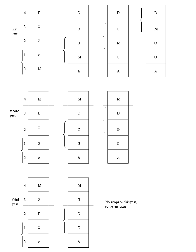
Bubblesort is based on swapping out-of-order pairs of data items, in sequence, so as to bubble to the top of the array (if pictured vertically) the largest data item. That largest item is somehow marked as done and the same game of bubbling the largest (of the rest of the data items) to the top is played all over again, etc. Thus we get the largest at the top, then the second largest, then the third largest, etc.

Although the psuedocode sorts an array of integers, for the purpose of tracing the workings of bubblesort let's pretend that we have modified it to sort an array of characters. This leads to the following drawings, where each row (or "pass") is handled by the for loop and the succession of passes is handled by the while loop. The bracket in each drawing of the array shows the two data items that are being compared to see if they are out of order.

We can see that a few improvements to the algorithm, such as an early exit, can allow Bubble Sort to take only N comparisons on N items when the data is already in the correctly sorted order. However, it is still normally the slowest of the three simple sorts. It only real advantage is that it has the simplest algorithm to code.

In the worst case (when the data is in descending order), every comparison will show that the data is out of order and thus result in a swap. In the worst case, then, the number of swaps equals the number of key comparisons. If the number of data items in the array is n, the number of swaps in the worst case is clearly (n-1) + (n-2) + ... + 3 + 2 + 1 = n*(n-1)/2 = n^2/2 - n/2, which is a Theta(n^2) function. Overall, bubblesort is known as a Theta(n^2) sort. Here is a summary:

Case	# Swaps	# Comparisons
Best	None	Ω( n)
Average	Ω( n^2)	Ω( n^2)
Worst	Ω( n^2)	Ω( n^2)

Even with an early exit, if the smallest value in the array is in location A[N], where A is an N item array to be sorted in ascending order, Bubble Sort still takes N² – 2N + 1 comparisons to sort the array. Because of this, there is a variation on Bubble Sort called Shaker Sort or Two-Way Bubble Sort that attempts to get around this problem. However, Shaker Sort also has a special case which will cause it to take N² – 2N + 1 comparisons: Place the middle element in the first position of the array and the rest of the data in descending order.

One of the reasons that both Insertion Sort and Bubble Sort are O( N² ) algorithms, is that they sort by exchanging adjacent elements. We can prove mathematically that in the general case a sorting algorithm that only exchanges adjacent elements can not do better than O( N² ). This means that a characteristic of an advanced sort, which does better than O( N² ), is that it exchanges elements that are not adjacent.

Insertion Sort:

We can see that the worst case for Insertion Sort is when the data is sorted in the opposite order; i.e., the data is in descending order and we want it sorted in ascending order. In this case, for N items, the sort requires, 1 + 2 + 3 + … + N -1 comparisons. By Gauss’s formula, this is ((N(N-1))/2)-N comparisons, which makes Insertion Sort an O( N²) algorithm. The best case for Insertion Sort, however, occurs when the data is already sorted in the proper order. In this case, the sort requires N comparisons for N data items making it an Ω(N) sort in the best case.

A variation of Insertion Sort is called Binary Insertion Sort. This sort uses a binary search to find the proper location for the item being inserted. However, while a binary insertion sort can take less time than insertion sort for a large array, the asymptotic run-time does not change.

Selection Sort:

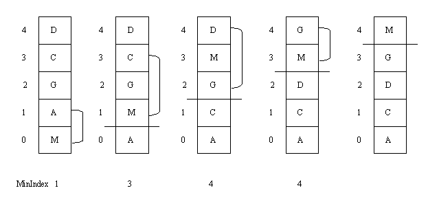
Another common sort routine is selection sort. The basic idea of the SelectionSort function is that it makes a pass through the array to find the index of the minimum item and then swaps that minimum item with the item at the bottom of the array. That bottom item is then marked as done. (This is shown in the drawing below by putting a solid line across.) Then the same game is played with the remaining items above that solid line: find the index of the minimum and swap it with the item at the bottom. By the time you reach the last picture in the drawing below, the smallest item is at index 0, the second smallest at index 1, etc. The only seemingly unchecked item is the one at the top, but it must be the largest by default. Thus the array has been sorted.


In the drawing above, the index of the minimum is shown below each picture of the array. A selection sort can also be based on finding the index of the maximum on each pass. Note that our SelectionSort function may on occasion end up swapping an item with itself. If you want, you can add an extra condition to check that the indices are different before attempting a swap.

As usual we can count the number of swaps or the number of key comparisons. The following chart shows the results:

Pass	# Swaps	# Comparisons
1	1	n-1
2	1	n-2
3	1	n-3
etc.
n-1	1	1

As we can see from the example, a selection sort must run a minimum or a maximum function on the unsorted portion of the data to find the next element to be placed. Since it takes N comparisons to find the minimum or the maximum of N unsorted items, selection sort requires N + N-1 + N-2 + … + 2 comparisons to sort N items. Again, by Gauss’s formula, this makes Selection Sort O( N² ). Note, however, that it doesn’t matter if the data is sorted already or not. Selection Sort requires the same number of comparisons in all cases, so that Selection Sort is Ω( N² ) as well.

---

---