Common Graph Algorithms
From
| ← Variations of Graph ADTs | ↑ Contents: CS2 | End |
Contents |
Graph Traversals
Graph breadth-first traversal is implemented using the same algorithm as with the tree ADT, with the addition that you have to check for nodes that have previously added to the work queue, usually by marking the node somehow. This requirement is needed as graphs may be cyclic; which would cause infinite looping in this algorithm without this check.
A Breadth-First Traversal has the following algorithm (for connected graphs):
Let Q be a queue that holds vertices (nodes) and let P be a pointer to a vertex (node).

Choose and enqueue a starting vertex from the graph.

WHILE the queue is not empty do the following

    dequeue a vertex and assign it to P
    visit the vertex pointed to by P

    FOREACH child of the vertex that has not been previously MARKED
        enqueue the child
    ENDFOR

ENDWHILE
A breadth-first traversal is often called a level-order traversal. Note that we can also change the above algorithm to a depth-first traversal by simply changing from a Queue to a Stack (and the enqueues/dequeues to pushes/pops)
Minimum Spanning Tree algorithms
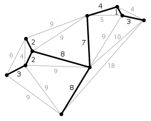
Given a connected graph, undirected graph, a spanning tree of that graph is a subgraph which is a tree and connects all the vertices together. A single graph can have many different spanning trees. We can also assign a weight to each edge, which is a number representing how unfavorable it is, and use this to assign a weight to a spanning tree by computing the sum of the weights of the edges in that spanning tree. A minimum spanning tree (MST) or minimum weight spanning tree is then a spanning tree with weight less than or equal to the weight of every other spanning tree. More generally, any undirected graph (not necessarily connected) has a minimum spanning forest, which is a union of minimum spanning trees for its connected components.
One example would be a cable TV company laying cable to a new neighborhood. If it is constrained to bury the cable only along certain paths, then there would be a graph representing which points are connected by those paths. Some of those paths might be more expensive, because they are longer, or require the cable to be buried deeper; these paths would be represented by edges with larger weights. A spanning tree for that graph would be a subset of those paths that has no cycles but still connects to every house. There might be several spanning trees possible. A minimum spanning tree would be one with the lowest total cost.
Prim's Algorithm
Prim's algorithm continuously increases the size of a tree starting with a single vertex until it spans all the vertices. Basically, this grows the tree, one vertex at a time by adding the least cost edge that connects a vertex that is not currently connected to the tree.
- Input: A connected weighted graph with vertices V and edges E.
- Initialize: Vnew = {x}, where x is an arbitrary node (starting point) from V, Enew = {}
- Repeat until Vnew = V:
- Choose edge (u,v) with minimal weight such that u is in Vnew and v is not (if there are multiple edges with the same weight, choose arbitrarily but consistently)
- Add v to Vnew, add (u, v) to Enew
- Output: Vnew and Enew describe a minimal spanning tree
Kruskal's algorithm
Kruskal's algorithm finds a minimum spanning tree for a connected weighted graph. This means it finds a subset of the edges that forms a tree that includes every vertex, where the total weight of all the edges in the tree is minimized. If the graph is not connected, then it finds a minimum spanning forest (a minimum spanning tree for each connected component). Kruskal's algorithm is an example of a greedy algorithm.
It works as follows:
- create a forest F (a set of trees), where each vertex in the graph is a separate tree
- create a set S containing all the edges in the graph
- while S is nonempty
- remove an edge with minimum weight from S
- if that edge connects two different trees, then add it to the forest, combining two trees into a single tree
- otherwise discard that edge.
At the termination of the algorithm, the forest has only one component and forms a minimum spanning tree of the graph.
This algorithm first appeared in Proceedings of the American Mathematical Society, pp. 48–50 in 1956, and was written by Joseph Kruskal.
Shortest Path algorithms
Dijkstra's algorithm, conceived by Dutch computer scientist Edsger Dijkstra in 1959, is a graph search algorithm that solves the single-source shortest path problem for a graph with nonnegative edge path costs, producing a shortest path tree. This algorithm is often used in routing.
For a given source vertex (node) in the graph, the algorithm finds the path with lowest cost (i.e. the shortest path) between that vertex and every other vertex. It can also be used for finding costs of shortest paths from a single vertex to a single destination vertex by stopping the algorithm once the shortest path to the destination vertex has been determined. For example, if the vertices of the graph represent cities and edge path costs represent driving distances between pairs of cities connected by a direct road, Dijkstra's algorithm can be used to find the shortest route between one city and all other cities. As a result, the shortest path first is widely used in network routing protocols, most notably IS-IS and OSPF (Open Shortest Path First).
Dijkstra's Algorithm
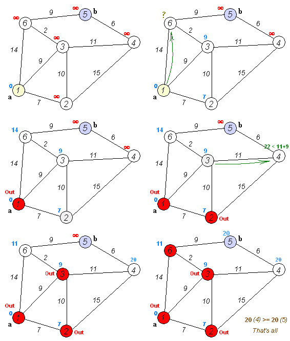
Let's call the node we are starting with an initial node. Let a distance of a node Y be the distance from the initial node to it. Dijkstra's algorithm will assign some initial distance values and will try to improve them step-by-step.
- Assign to every node a distance value. Set it to zero for our initial node and to infinity for all other nodes.
- Mark all nodes as unvisited. Set initial node as current.
- For current node, consider all its unvisited neighbours and calculate their distance (from the initial node). For example, if current node (A) has distance of 6, and an edge connecting it with another node (B) is 2, the distance to B through A will be 6+2=8. If this distance is less than the previously recorded distance (infinity in the beginning, zero for the initial node), overwrite the distance.
- When we are done considering all neighbours of the current node, mark it as visited. A visited node will not be checked ever again; its distance recorded now is final and minimal.
- Set the unvisited node with the smallest distance (from the initial node) as the next "current node" and continue from step 3
In graph theory, the shortest path problem is the problem of finding a path between two vertices (or nodes) such that the sum of the weights of its constituent edges is minimized. An example is finding the quickest way to get from one location to another on a road map; in this case, the vertices represent locations and the edges represent segments of road and are weighted by the time needed to travel that segment.
Formally, given a weighted graph (that is, a set V of vertices, a set E of edges, and a real-valued weight function f : E → 'R), and one element v of V, find a path P from v to each v of V so that

is minimal among all paths connecting v to v' .
The problem is also sometimes called the single-pair shortest path problem, to distinguish it from the following generalizations:
- The single-source shortest path problem, in which we have to find shortest paths from a source vertex v to all other vertices in the graph.
- The single-destination shortest path problem, in which we have to find shortest paths from all vertices in the graph to a single destination vertex v. This can be reduced to the single-source shortest path problem by reversing the edges in the graph.
- The all-pairs shortest path problem', in which we have to find shortest paths between every pair of vertices v, v in the graph.
These generalizations have significantly more efficient algorithms than the simplistic approach of running a single-pair shortest path algorithm on all relevant pairs of vertices.
Applications of Shortest Path Algrithms
Shortest path algorithms are applied to automatically find directions between physical locations, such as driving directions on web mapping websites like Mapquest or Google Maps.
If one represents a nondeterministic abstract machine as a graph where vertices describe states and edges describe possible transitions, shortest path algorithms can be used to find an optimal sequence of choices to reach a certain goal state, or to establish lower bounds on the time needed to reach a given state. For example, if vertices represents the states of a puzzle like a Rubik's Cube and each directed edge corresponds to a single move or turn, shortest path algorithms can be used to find a solution that uses the minimum possible number of moves.
In a networking or telecommunications mindset, this shortest path problem is sometimes called the min-delay path problem and usually tied with a widest path problem. For example, the algorithm may seek the shortest (min-delay) widest path, or widest shortest (min-delay) path.
A more lighthearted application is the games of "Six degrees of separation|Six degrees of separation" that try to find the shortest path in graphs like movie stars appearing in the same film.
Other applications include "operations research, plant and facility layout, robotics, transportation, and Very-large-scale integration design".<ref>Danny Z. Chen. Developing Algorithms and Software for Geometric Path Planning Problems. ACM Computing Surveys 28A(4), December 1996.</ref>
Travelling Salesman Problem

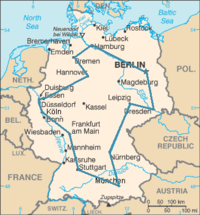
The Travelling Salesman Problem (TSP) is a problem in combinatorial optimization studied in operations research and theoretical computer science. Given a list of cities and their pairwise distances, the task is to find a shortest possible tour that visits each city exactly once.
The problem was first formulated as a mathematical problem in 1930 and is one of the most intensively studied problems in optimization. It is used as a benchmark for many optimization methods. Even though the problem is computationally difficult, a large number of heuristics and exact methods are known, so that some instances with tens of thousands of cities can be solved.
The TSP has several applications even in its purest formulation, such as planning, logistics, and the manufacture of Integrated circuits. Slightly modified, it appears as a sub-problem in many areas, such as DNA sequencing. In these applications, the concept city represents, for example, customers, soldering points, or DNA fragments, and the concept distance represents travelling times or cost, or a similarity measure between DNA fragments. In many applications, additional constraints such as limited resources or time windows make the problem considerably harder.
In the theory of computational complexity, the decision version of TSP belongs to the class of NP-complete problems. Thus, it is assumed that there is no efficient algorithm for solving TSPs. In other words, it is likely that the worst case running time for any algorithm for TSP increases exponentially with the number of cities, so even some instances with only hundreds of cities will take many CPU years to solve exactly.
Description as a graph problem
TSP can be modeled as a graph, such that cities are the graph's vertices, paths are the graph's edges, and a path's distance is the edge's length. A TSP tour becomes a Hamiltonian cycle, and the optimal TSP tour is the shortest Hamiltonian cycle. Often, the model is a complete graph (i.e., an edge connects each pair of vertices). If no path exists between two cities, adding an arbitrarily long edge will complete the graph without affecting the optimal tour.
Computing a solution
The traditional lines of attack for the NP-hard problems are the following:
- Devising algorithms for finding exact solutions (they will work reasonably fast only for relatively small problem sizes).
- Devising "suboptimal" or heuristic algorithms, i.e., algorithms that deliver either seemingly or probably good solutions, but which could not be proved to be optimal.
- Finding special cases for the problem ("subproblems") for which either better or exact heuristics are possible.
Computational complexity
The problem has been shown to be NP-hard (more precisely, it is complete for the complexity class FPNP; see function problem), and the decision problem version ("given the costs and a number x, decide whether there is a round-trip route cheaper than x") is NP-complete. The bottleneck traveling salesman problem is also NP-hard. The problem remains NP-hard even for the case when the cities are in the plane with Euclidean distances, as well as in a number of other restrictive cases. Removing the condition of visiting each city "only once" does not remove the NP-hardness, since it is easily seen that in the planar case there is an optimal tour that visits each city only once (otherwise, by the triangle inequality, a shortcut that skips a repeated visit would not increase the tour length).
Complexity of approximation
In the general case, finding a shortest travelling salesman tour is NPO-complete.[2] If the distance measure is a metric and symmetric, the problem becomes APX-complete[3] and Christofides’s algorithm approximates it within 3/2.[4] If the distances are restricted to 1 and 2 (but still are a metric) the approximation ratio becomes 7/6. In the asymmetric, metric case, only logarithmic performance guarantees are known, the best current algorithm achieves performance ratio 0.814 log n;[5] it is an open question if a constant factor approximation exists.
The corresponding maximization problem of finding the longest travelling salesman tour is approximable within 63/38.[6] If the distance function is symmetric, the longest tour can be approximated within 4/3 by a deterministic algorithm [7] and within (33 + ε) / 25 by a randomised algorithm.[8]
Exact algorithms
The most direct solution would be to try all permutations (ordered combinations) and see which one is cheapest (using brute force search). The running time for this approach lies within a polynomial factor of O(n!), the factorial of the number of cities, so this solution becomes impractical even for only 20 cities. One of the earliest applications of dynamic programming is an algorithm that solves the problem in time O(n22n).[9]
The dynamic programming solution requires exponential space. Using inclusion–exclusion, the problem can be solved in time within a polynomial factor of 2n and polynomial space.[10]
Improving these time bounds seems to be difficult. For example, it is an open problem if there exists an exact algorithm for TSP that runs in time O(1.9999n)[11]
Other approaches include:
- Various Branch and bound|branch-and-bound algorithms, which can be used to process TSPs containing 40-60 cities.
- Progressive improvement algorithms which use techniques reminiscent of linear programming. Works well for up to 200 cities.
- Implementations of branch-and-bound and problem-specific cut generation; this is the method of choice for solving large instances. This approach holds the current record, solving an instance with 85,900 cities, see [12]
Heuristic and approximation algorithms
Various heuristics and approximation algorithms, which quickly yield good solutions have been devised. Modern methods can find solutions for extremely large problems (millions of cities) within a reasonable time which are with a high probability just 2-3% away from the optimal solution.
CS2: Data Structures
Theory of Computation - ADT Preliminaries
Linear ADTs - Tree ADTs - Graph ADTs - Unordered Collection ADTs


